Dynamatic
Dynamatic is an academic, open-source high-level synthesis compiler that produces synchronous dynamically-scheduled circuits from C/C++ code. Dynamatic generates synthesizable RTL which currently targets Xilinx FPGAs and delivers significant performance improvements compared to state-of-the-art commercial HLS tools in specific situations (e.g., applications with irregular memory accesses or control-dominated code). The fully automated compilation flow of Dynamatic is based on MLIR. It is customizable and extensible to target different hardware platforms and easy to use with commercial tools such as Vivado (Xilinx) and Modelsim (Mentor Graphics).
We welcome contributions and feedback from the community. If you would like to participate, please check out our contribution guidelines
Using Dynamatic
To get started using Dynamatic (after setting it up), check out our introductory tutorial, which guides you through your first compilation of C code into a synthesizable dataflow circuit! If you want to start modifying Dynamatic and are new to MLIR or compilers in general, our MLIR primer and pass creation tutorial will help you take your first steps.
Setting up Dynamatic
There are currently two ways to setup and use Dynamatic
1. Build From Source (Recommended)
We support building from source on Linux and on Windows (through WSL). See our Build instructions below. Ubuntu 24.04 LTS is officially supported; other apt-based distributions should work as well. Other distributions may also require cosmetic changes to the dependencies you have to install before running Dynamatic.
2. Use the Provided Virtual Machine
We provide an Ubuntu-based Virtual Machine (VM) that already has Dynamatic and our dataflow circuit visualizer set up. You can use it to simply follow the tutorial (Using Dynamatic) or as a starting point to use/modify Dynamatic in general.
Build Instructions
The following instructions can be used to setup Dynamatic from source.
note
If you intend to modify Dynamatic’s source code and/or build the interactive dataflow circuit visualizer (recommended for circuit debugging), you can check our advanced build instructions to learn how to customize the build process to your needs.
1. Install Dependencies Required by the Project
Most of our dependencies are provided as standard packages on most Linux distributions. Dynamatic needs a working C/C++ toolchain (compiler, linker), cmake and ninja for building the project, Python (3.6 or newer), GraphViz to work with .dot files, and standard command-line tools like git.
On apt-based Linux distributions:
apt-get update
apt-get install clang lld ccache cmake ninja-build python3 graphviz git curl gzip libreadline-dev libboost-all-dev
Note that you may need super user privileges for any package installation. You can use sudo before entering the commands
clang, lld, and ccache are not strictly required but significantly speed up (re)builds. If you do not wish to install them, call the build script with the –disable-build-opt flag to prevent their usage.
Dynamatic utilizes Gurobi to optimize the circuit’s performance. It is optional and Dynamatic will build properly without it but is useful for more optimized results. Refer to our Advanced Build page for guidance on how to setup the Gurobi solver.
tip
While this section helps you install the dependencies needed to get started with Dynamatic, you can find a list of dependencies used by Dynamatic in the dependencies section for a better understanding of how the tool works.
Finally, Dynamatic uses Modelsim or Questa to run simulations.
These are optional tools which you can see how to install in the Advanced Build page if you intend to use the simulator.
tip
Before moving on to the next step, refresh your environment variables in your current terminal to make sure that all newly installed tools are visible in your PATH. Alternatively, open a new terminal and proceed to cloning the project.
2. Cloning the Project and Its Submodules
Dynamatic depends on a fork of LLVM/MLIR. To instruct git to clone the appropriate versions submodules used by Dynamatic, we enable the --recurse-submodules flag.
git clone --recurse-submodules https://github.com/EPFL-LAP/dynamatic.git
This creates a dynamatic folder in your current working directory.
3. Build the Project
Run the build script from the directory created by the clone command (see the advanced build instructions for details on how to customize the build process).
cd dynamatic
chmod +x ./build.sh
./build.sh --release
Using prebuilt LLVM. The commands above might take quite some time to finish since we need to build LLVM. Alternatively, the build.sh script can download a prebuilt LLVM and link Dynamatic against that instead. If this is preferred, you could run the following command:
./build.sh --release --use-prebuilt-llvm
note
You need at least 6GB of free disk space for Dynamatic (if you enable the --use-prebuilt-llvm option).
If you need to build llvm-project from scratch, you will need at least 50GB
of free disk space and 16GB+ of RAM.
4. Run the Dynamatic Testsuite
To confirm that you have successfully compiled Dynamatic and to test its functionality, you can run Dynamatic’s testsuite from the top-level build folder using ninja.
# From the "dynamatic" folder created by the clone command
cd build
ninja check-dynamatic
You can now launch the Dynamatic front-end from Dynamatic’s top level directory using:
./bin/dynamatic
With Dynamatic correctly installed, you can browse the using dynamatic tutorial to learn how to use the basic commands and features in Dynamatic to convert your C code into RTL.
You can also explore the Advanced build options.
Tutorials
Welcome to the Dynamatic tutorials!
To encourage contributions to the project, we aim to support newcomers to the worlds of software development and compilers by providing development tutorials that can help them take their first steps inside the codebase. They are mostly aimed at people who have no or little compiler development experience, especially with the MLIR compiler infrastructure with which Dynamatic is deeply intertwined. Some prior knowledge of C++ (more generally, of object-oriented programming) and of the theory behind dataflow circuits is assumed.
Introduction to Dynamatic
This two-part tutorial first introduces the toolchain and teaches you to use the Dynamatic frontend to synthesize, simulate, and visualize dataflow circuits compiled from C code. The second part guides you through the creation of a small compiler optimization pass and gives you some insight into how the toolchain can help you identify issues in your circuits. This tutorial is a good starting point for anyone wanting to get into Dynamatic, without necessarily modifying it.
The MLIR Primer
This tutorial, heavily based on MLIR’s official language reference, is meant as a quick introduction to MLIR and its core constructs. C++ code snippets are peperred through the tutorial in an attempt to ease newcomers to the framework’s C++ API and provide some initial code guidance.
Creating Compiler Passes
This tutorial goes through the creation of a simple compiler transformation pass that operates on Handshake-level IR (i.e., on dataflow circuits modeled in MLIR). It goes into details into all the code that one needs to write to declare a pass in the codebase, implement it, and then run it on some input code using the dynamatic-opt tool. It then touches on different ways to write the same pass as to give an idea of MLIR’s code transformation capabilities.
Introduction to Dynamatic
This tutorial is meant as the entry-point for new Dynamatic users and will guide you through your first interactions with the compiler and its surrounding toolchain. Following it requires that you have Dynamatic built locally on your machine, either from source or using our custom virtual machine (VM setup instructions).
warning
Note that the virtual machine does not contain an MILP solver; when using frontend scripts, you will have to provide the --simple-buffers flag to the compile command to instruct it to not rely on an MILP solver for buffer placement. Unfortunately, this will affect the circuits you generate as part of the exercises and you may therefore obtain different results from what the tutorial describes.
It is divided in the following two chapters.
- Chapter #1 - Using Dynamatic | We use Dynamatic’s frontend to synthesize our first dataflow circuit from C code, then visualize it using our interactive dataflow visualizer.
- Chapter #2 - Modifying Dynamatic | We write a small compiler transformation pass in C++ to try to improve circuit performance and decrease area, then debug it using the visualizer.
Running an Integration Test
1. Binary Search
This example describes how to use Dynamatic and become more familiarized with its HLS flow. You will see how:
- compile your C code to RTL
- simulate the resulting circuit using ModelSim
- synthesize your circuit using vivado
- visualize your circuit
Source Code
//===- binary_search.c - Search for integer in array  -------------*- C -*-===//
//
// Implements the binary_search kernel.
//
//===----------------------------------------------------------------------===//

#include "binary_search.h"
#include "dynamatic/Integration.h"

int binary_search(in_int_t search, in_int_t a[N]) {
  int evenIdx = -1;
  int oddIdx = -1;

  for (unsigned i = 0; i < N; i += 2) {
    if (a[i] == search) {
      evenIdx = (int)i;
      break;
    }
  }

  for (unsigned i = 1; i < N; i += 2) {
    if (a[i] == search) {
      oddIdx = (int)i;
      break;
    }
  }

  int done = -1;
  if (evenIdx != -1)
    done = evenIdx;
  else if (oddIdx != -1)
    done = oddIdx;

  return done;
}

int main(void) {
  in_int_t search = 55;
  in_int_t a[N];
  for (int i = 0; i < N; i++)
    a[i] = i;
  CALL_KERNEL(binary_search, search, a);
  return 0;
}
This HLS code includes control flow inside loops, limiting pipelining in statically scheduled HLS due to worst-case assumptions—here, the branch is taken and the loop exits early. Dynamically scheduled HLS, like Dynamatic, adapts to runtime behavior. Let’s see how the generated circuit handles control flow more flexibly.
Launching Dynamatic
If you haven’t added Dynamatic to path, navigate to the directory where you cloned Dynamatic and run the command below:
./bin/dynamatic
The Dynamatic frontend would be displayed as follows
username:~/Dynamatic/dynamatic$ ./bin/dynamatic
================================================================================
============== Dynamatic | Dynamic High-Level Synthesis Compiler ===============
======================== EPFL-LAP - v2.0.0 | March 2024 ========================
================================================================================


dynamatic>
Set the Path to the C Target C File
Use the set-src command to direct Dynamatic to the file you want to synthesize into RTL
dynamatic> set-src integration-test/binary_search/binary_search.c
Compile the C File to a Lower Intermediate Representation
You can choose the buffer placement algorithm with the --buffer-algorithm flag. For this example, we use fpga20, a throughput driven algorithm which requires Gurobi installed as describe in the Advanced Build page.
tip
If you are not sure which options are available for the compile command, add anything after it and hit enter to see the options e.g compile –
dynamatic> compile --buffer-algorithm fpga20
[INFO] Compiled source to affine
[INFO] Ran memory analysis
[INFO] Compiled affine to scf
[INFO] Compiled scf to cf
[INFO] Applied standard transformations to cf
[INFO] Applied Dynamatic transformations to cf
[INFO] Compiled cf to handshake
[INFO] Applied transformations to handshake
[INFO] Built kernel for profiling
[INFO] Ran kernel for profiling
[INFO] Profiled cf-level
[INFO] Running smart buffer placement with CP = 4.000 and algorithm = 'fpga20'
[INFO] Placed smart buffers
[INFO] Canonicalized handshake
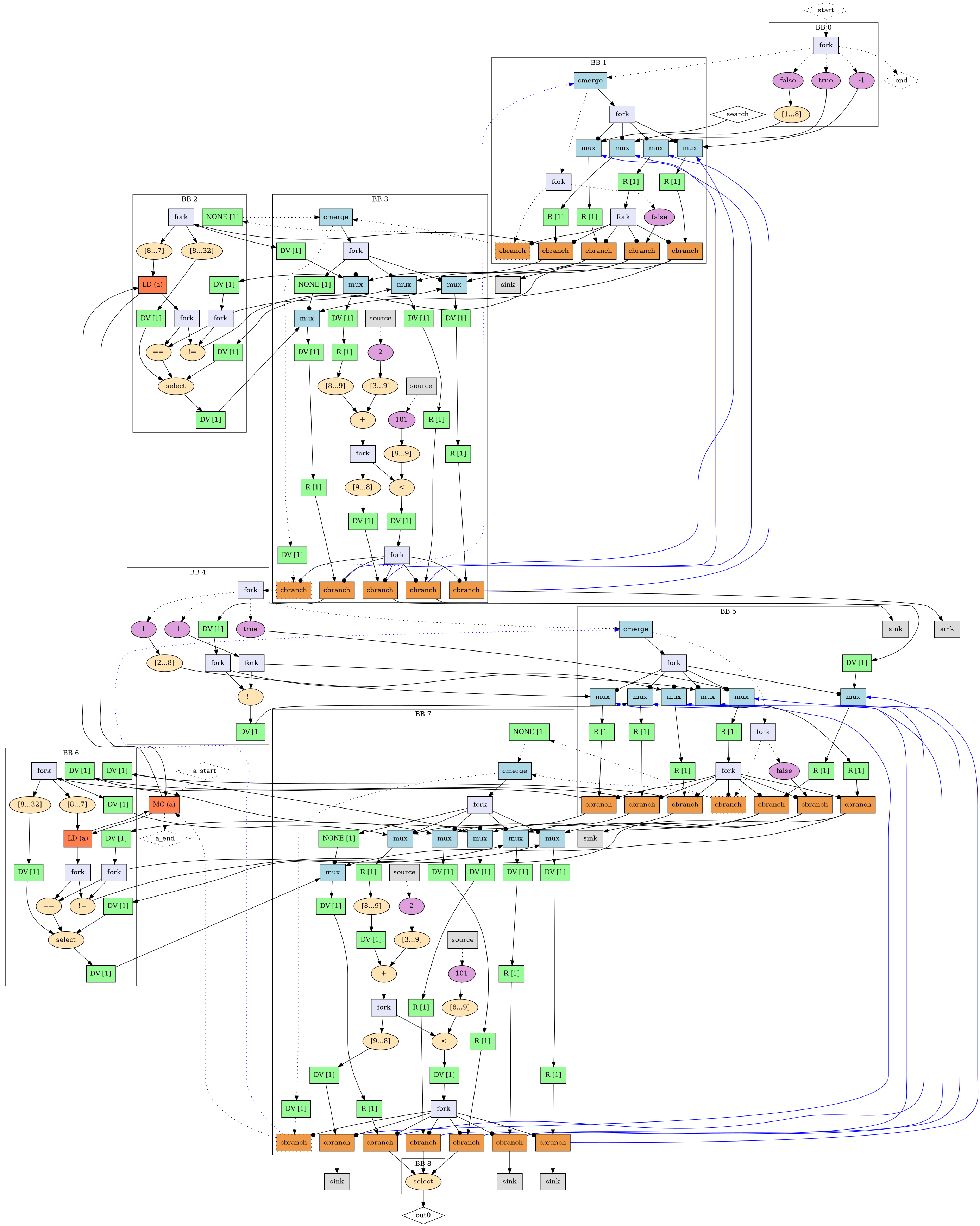
[INFO] Created binary_search DOT
[INFO] Converted binary_search DOT to PNG
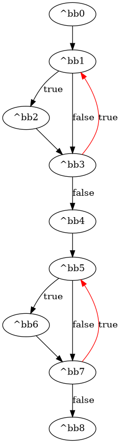
[INFO] Created binary_search_CFG DOT
[INFO] Converted binary_search_CFG DOT to PNG
[INFO] Lowered to HW
[INFO] Compilation succeeded
tip
Two PNG files are generated at compile time, kernel_name.png and kernel_name_CFG.png, allowing you to have a preview of your circuit and its control flow graph generated by Dynamatic as shown below.
Binary Search CFG
Binary Search Dataflow Circuit
Generate HDL from mlir File
An mlir file is generated during the compile process.
write-hdl converts it into HDL code for your kernel. The default HDL is VHDL. You can choose verilog or vhdl with the --hdl flag
dynamatic> write-hdl --hdl vhdl
[INFO] Exported RTL (vhdl)
[INFO] HDL generation succeeded
Simulate Your Circuit
This step simulates the kernel in C and HDL (using modelsim) and compares the results for equality.
dynamatic> simulate
[INFO] Built kernel for IO gen.
[INFO] Ran kernel for IO gen.
[INFO] Launching Modelsim simulation
[INFO] Simulation succeeded
Sythesize With Vivado
This step is optional. It allows to get more timing and performance related files using vivado. You must have vivado installed.
dynamatic> synthesize
[INFO] Created synthesis scripts
[INFO] Launching Vivado synthesis
[INFO] Logic synthesis succeeded
note
If this step fails despite you having vivado installed and added to path, source the vivado/vitis settings64.sh in your shell and try again.
warning
Adding the sourcing of the settings64.sh to path may hinder future compilations as the vivado compiler varies from the regular clang compiler on your machine
Visualize and Simulate Your Circuit
By running the visualize command, the Godot GUI will be launched with your dataflow circuit open, and ready to be played with
dynamatic> visualize
[INFO] Generated channel changes
[INFO] Added positioning info. to DOT
[INFO] Launching visualizer...
Below is a preview of the circuit in the Godot visualizer
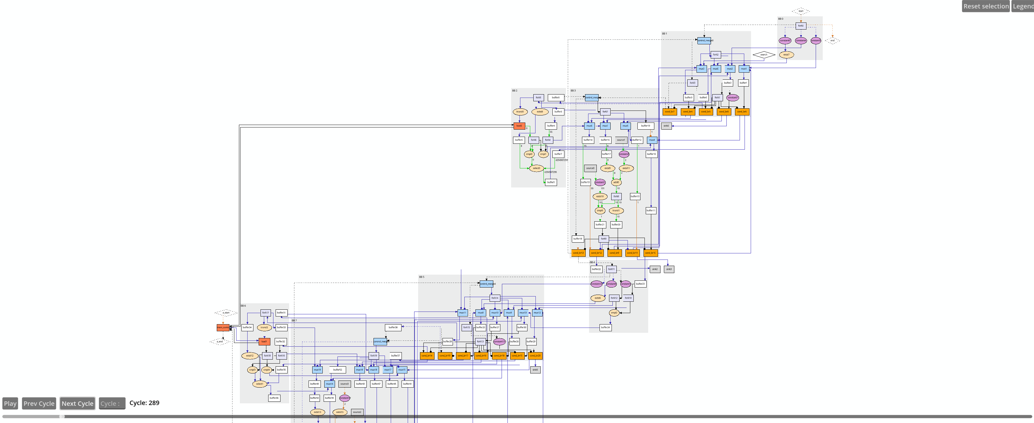 The circuit is too broad to capture in one image but you can move around the preview by clicking, holding, and moving your cursor around. Play with the commands to see your circuit in action.
Modifying Dynamatic
This tutorial logically follows the Using Dynamatic tutorial, and as such requires that you are already familiar with the concepts touched on in the latter. In this tutorial, we will write a small compiler optimization pass in C++ that will transform dataflow muxes into merges in an attempt to optimize our circuits’ area and throughput. While we will write a little bit of C++ in this tutorial, it does not require much knowledge in the language.
Below are some technical details about this tutorial.
- All resources are located in the repository’s
tutorials/Introduction/folder. Data exclusive to this chapter is located in theCh2subfolder, but we will also reuse data from the previous chapter,Ch1. - All relative paths mentionned throughout the tutorial are assumed to start at Dynamatic’s top-level folder.
- We assume that you have already built Dynamatic from source using the instructions in the Installing Dynamatic page or that you have access to a Docker container that has a pre-built version of Dynamatic .
This tutorial is divided into the following sections.
- Spotting an Optimization Opportunity | We take another look at the circuit from the previous tutorial and spot something that looks optimizable.
- Writing a Small Compiler Pass | We implement the optimization as a compiler pass, and add it the compilation script to use it.
- Testing Our Pass | We test our pass to make sure it works as intended, and find out that it may not.
- A problem, and a Solution! | After identifying a problem in one of our circuits, we implement a quick-and-dirty fix to make the circuit correct again.
- Conclusion | We reflect on everything we just accomplished.
Spotting an Optimization Opportunity
Let’s start by re-considering the same loop_multiply kernel (Ch1/loop_multiply.c) from the previous tutorial. See its definition below.
// The kernel under consideration
unsigned loop_multiply(in_int_t a[N]) {
  unsigned x = 2;
  for (unsigned i = 0; i < N; ++i) {
    if (a[i] == 0)
      x = x * x;
  }
  return x;
}
This simple kernel multiplies a number by itself at each iteration of a simple loop from 0 to any number N where the corresponding element of an array equals 0. The function returns the calculated value after the loop exits.
If you have deleted the data generated by the synthesis flow on this kernel, you can regenerate it fully using the loop-multiply.dyn frontend script (Ch2/loop-multiply.dyn) that has already been written for you. Just run the following command from Dynamatic’s top-level folder.
./bin/dynamatic --run tutorials/Introduction/Ch2/loop-multiply.dyn
This will compile the C kernel, functionally verify the generated VHDL, and re-open the dataflow visualizer. Note the [INFO] Simulation succeeded message in the output (after the simulate command), indicating that outputs of the VHDL design matched those of the original C kernel. All output files are generated in tutorials/Introduction/usingDynamatic/out.
tip
Identify all muxes in the circuit and derive their purpose in this circuit. Remember that muxes have an arbitrary number of data inputs (here it is always 2) and one select input, which selects which valid data input gets forwarded to the output. Note that, in general, the select input of muxes if generated by the index output of the same block’s control merge.
Another dataflow component that is similar to the mux in purpose is the merge. Identically to the mux, the merge has an arbitrary number of data inputs, one of which gets forwarded to the output when it is valid. However, the two dataflow components have two key differences.
- The merge does not have a
selectinput. Instead, at any given cycle, if any of its data input is valid and if its data output is ready, it will transfer a token to the output. - The merge does not provide any guarantee on input consumption order if at any given cycle multiple of its inputs are valid and its data output if ready. In those situations, it will simply transfer one of its input tokens to its output.
Due to this “simpler” interface, a merge is generally smaller in area than a corresponding mux with the same number of data inputs. Replacing a mux with a merge may also speed up circuit execution since the merge does not have to wait for the arrival of a valid select token to transfer one of its data inputs to its output.
Let’s try to make this circuit smaller by writing a compiler pass that will automatically replace all muxes with equivalent merges then!
Writing a Small Compiler Pass
In this section, we will add a small transformation pass that achieves the optimization opportunity we identified in the previous section. We will not go into much details into how C++ or MLIR works, our focus will be instead in writing something minimal that accomplishes the job cleanly. For a more complete tutorial on pass-writing, feel free to go through the “Creating Passes” tutorial after completing this one.
Creating this pass will involve creating 2 new source files and making minor editions to 3 existing source files. In order, we will
- Declare the Pass in TableGen (a LLVM/MLIR language that eventually transpiles to C++).
- Write a Minimal C++ Header for the Pass.
- Implement the Pass in C++.
- Make New Source File We Created Part of Dynamatic’s Build Process.
- Edit a Generic Header to Make Our Pass Visible to Dynamatic’s Optimizer.
Declaring the Pass in TableGen
The first thing we need to do is declare our pass somewhere. In LLVM/MLIR, this happens in the TableGen language, a declarative format that ultimately transpiles to C++ during the build process to automatically generate a lot of boilerplate C++ code.
Open the include/dynamatic/Transforms/Passes.td file and copy-and-paste the following snippet anywhere below the include lines at the top of the file.
def HandshakeMuxToMerge : DynamaticPass<"handshake-mux-to-merge"> {
  let summary = "Transform all muxes into merges.";
  let description = [{
    Transform all muxes within the IR into merges with identical data operands.
  }];
  let constructor = "dynamatic::createHandshakeMuxToMerge()";
}
This declares a compiler pass whose C++ class name will be based on HandshakeMuxToMerge and which can be called using the --handshake-mux-to-merge flag from Dynamatic’s optimizer (we will go into more details into using Dynamatic’s optimizer in the “Testing our pass” section). The summary and description fields are optional but useful to describe the pass’s purpose. Finally, the constructor field indicates the name of a C++ function that should returns an instance of our pass. We will declare and then define this method in the next two subsections.
A Minimal C++ Header for the Pass
We now need to write a small C++ header for our new pass. Each pass has one, and they are for the large part always structured in the same exact way. Create a file in include/dynamatic/Transforms called HandshakeMuxToMerge.h and paste the following chunk of code into it:
/// Classical C-style header guard
#ifndef DYNAMATIC_TRANSFORMS_HANDSHAKEMUXTOMERGE_H
#define DYNAMATIC_TRANSFORMS_HANDSHAKEMUXTOMERGE_H

/// Include some basic headers
#include "dynamatic/Support/DynamaticPass.h"
#include "dynamatic/Support/LLVM.h"
#include "mlir/Pass/Pass.h"

namespace dynamatic {

/// The following include file is autogenerated by LLVM/MLIR during the build
/// process from the Passes.td file we just edited. We only want to include the
/// part of the file that refers to our pass (it contains delcaration code for
/// all transformation passes), which we select using the two macros below.
#define GEN_PASS_DECL_HANDSHAKEMUXTOMERGE
#define GEN_PASS_DEF_HANDSHAKEMUXTOMERGE
#include "dynamatic/Transforms/Passes.h.inc"

/// The pass constructor, with the same name we specified in TableGen in the
/// previous subsection.
std::unique_ptr<dynamatic::DynamaticPass> createHandshakeMuxToMerge();

} // namespace dynamatic

#endif // DYNAMATIC_TRANSFORMS_HANDSHAKEMUXTOMERGE_H
This file does two important things:
- It includes C++ code auto-generated from the
Passes.tdfile we just edited. - It declares the pass header that we announced in the pass’s TableGen declaration.
Now that all declarations are made, it is time to actually implement our IR transformation!
Implementing the Pass
Create a file in lib/Transforms called HandshakeMuxToMerge.cpp and in which we will implement our pass. Paste the following code into it:
/// Include the header we just created.
#include "dynamatic/Transforms/HandshakeMuxToMerge.h"

/// Include some other useful headers.
#include "dynamatic/Dialect/Handshake/HandshakeOps.h"
#include "dynamatic/Support/CFG.h"
#include "mlir/Transforms/GreedyPatternRewriteDriver.h"

using namespace dynamatic;

namespace {

/// Simple driver for the pass that replaces all muxes with merges.
struct HandshakeMuxToMergePass
    : public dynamatic::impl::HandshakeMuxToMergeBase<HandshakeMuxToMergePass> {

  void runDynamaticPass() override {
    // This is the top-level operation in all MLIR files. All the IR is nested
    // within it
    mlir::ModuleOp mod = getOperation();
    MLIRContext *ctx = &getContext();

    // Define the set of rewrite patterns we want to apply to the IR
    RewritePatternSet patterns(ctx);

    // Run a greedy pattern rewriter on the entire IR under the top-level module
    // operation
    mlir::GreedyRewriteConfig config;
    if (failed(applyPatternsAndFoldGreedily(mod, std::move(patterns), config))) {
      // If the greedy pattern rewriter fails, the pass must also fail
      return signalPassFailure();
    }
  };
};
}; // namespace

/// Implementation of our pass constructor, which just returns an instance of
/// the `HandshakeMuxToMergePass` struct.
std::unique_ptr<dynamatic::DynamaticPass>
dynamatic::createHandshakeMuxToMerge() {
  return std::make_unique<HandshakeMuxToMergePass>();
}
This file, at the botton, implements the pass constructor we declared in the header. This constuctor returns an instance of a struct defined just above—do not mind the slightly convoluted struct declaration, which showcases the curiously recurring template pattern C++ idiom that is used extensively throuhgout MLIR/Dynamatic—whose single method runDynamaticPass defines what happens when the pass is called. In our case, we want to leverage MLIR’s greedy pattern rewriter infrastructure to match on all muxes in the IR and replace them with merges with identical data inputs. If you would like to know more about how greedy pattern rewriting works, feel free to check out MLIR’s official documentation on the subject. For this simple pass, you do not need to understand exactly how it works, just that it can match and try to rewrite certain operations inside the IR based on a set of user-provided rewrite patterns. Speaking of rewrite patterns, let’s add our own to the file just above the HandshakeMuxToMergePass struct definition. Paste the following into the file.
/// Rewrite pattern that will match on all muxes in the IR and replace each of
/// them with a merge taking the same inputs (except the `select` input which
/// merges do not have due to their undeterministic nature).
struct ReplaceMuxWithMerge : public OpRewritePattern<handshake::MuxOp> {
  using OpRewritePattern<handshake::MuxOp>::OpRewritePattern;

  LogicalResult matchAndRewrite(handshake::MuxOp muxOp,
                                PatternRewriter &rewriter) const override {
    // Retrieve all mux inputs except the `select`
    ValueRange dataOperands = muxOp.getDataOperands();
    // Create a merge in the IR at the mux's position and with the same data
    // inputs (or operands, in MLIR jargon)
    handshake::MergeOp mergeOp =
        rewriter.create<handshake::MergeOp>(muxOp.getLoc(), dataOperands);
    // Make the merge part of the same basic block (BB) as the mux
    inheritBB(muxOp, mergeOp);
    // Retrieve the merge's output (or result, in MLIR jargon)
    Value mergeResult = mergeOp.getResult();
    // Replace usages of the mux's output with the new merge's output
    rewriter.replaceOp(muxOp, mergeResult);
    // Signal that the pattern succeeded in rewriting the mux
    return success();
  }
};
This rewrite pattern, called ReplaceMuxWithMerge, matches on operations of type handshake::MuxOp (the mux operation is part of the Handshake dialect) as indicated by its declaration. Eahc time the greedy pattern rewriter finds a mux in the IR, it will call the pattern’s matchAndRewrite method, providing it with the particular operation it matched on as well as with a PatternRewriter object to allow us to modify the IR. For this simple pass, we want to transform all muxes into merges so the rewrite pattern is very short:
- First, we extract the mux’s data inputs.
- Then, we create a merge operation at the same location in the IR and with the same data inputs.
- Finally, we tell the rewriter to replace the mux with the merge. This “rewires” the IR by making users of the mux’s output channel use the merge’s output channel instead, and deleted the original mux.
To complete the pass implementation, we simply have to provide the rewrite pattern to the greedy pattern rewriter. Just add the following call to patterns.add inside runDynamaticPass after declaring the pattern set.
RewritePatternSet patterns(ctx);
patterns.add<ReplaceMuxWithMerge>(ctx);
Congratulations! You have now implemented your first Dynamatic pass. We just have two simple file edits to make before we can start using it.
Adding our Pass to the Build Process
We need to make the build process aware of the new source file we just wrote. Navigate to lib/Transforms/CMakeLists.txt and add the name of thefile you created in the previous section next to other .cpp files in the add_dynamatic_library statement.
add_dynamatic_library(DynamaticTransforms
  HandshakeMuxToMerge.cpp # Add this line
  ArithReduceStrength.cpp
  ... # other .cpp files

  DEPENDS
  ...
)
Making our Pass Visible
Finally, we need to make Dynamatic’s optimizer aware of our new pass. Navigate to include/dynamatic/Transforms/Passes.h and add the header you wrote a couple of subsections ago to the list of include files.
#ifndef DYNAMATIC_TRANSFORMS_PASSES_H
#define DYNAMATIC_TRANSFORMS_PASSES_H

#include "dynamatic/Transforms/HandshakeMuxToMerge.h" // Add this line
... // other include files
Testing our Pass
Now that the pass is part of the project’s source code, we just have to partially re-build Dynamatic to use it. Simply navigate to the top-level build directory from the terminal and run ninja.
cd build && ninja && cd ..
If you see Build successfull printed on the terminal, then everything worked and the pass is now part of Dynamatic. Let’s go modify our compilation script—which is called by the frontend’s compile command—to run it as part of the normal synthesis flow.
Open tools/dynamatic/scripts/compile.sh and locate the following call to Dynamatic’s optimizer:
# handshake transformations
"$DYNAMATIC_OPT_BIN" "$F_HANDSHAKE" \
  --handshake-minimize-lsq-usage \
  --handshake-concretize-index-type="width=32" \
  --handshake-minimize-cst-width --handshake-optimize-bitwidths="legacy" \
  --handshake-materialize --handshake-infer-basic-blocks \
  > "$F_HANDSHAKE_TRANSFORMED"
exit_on_fail "Failed to apply transformations to handshake" \
  "Applied transformations to handshake"
This is a compilation step where we apply a number of optimizations/transformation to our Handshake-level IR for performance and correctness, and is thus a perfect place to insert our new pass. Remember that we declared our pass in Tablegen to be associated with the --handshake-mux-to-merge optimizer flag. We just have to add the flag to the optimizer call to run our new pass.
# handshake transformations
"$DYNAMATIC_OPT_BIN" "$F_HANDSHAKE" \
  --handshake-mux-to-merge \
  --handshake-minimize-lsq-usage \
  --handshake-concretize-index-type="width=32" \
  --handshake-minimize-cst-width --handshake-optimize-bitwidths="legacy" \
  --handshake-materialize --handshake-infer-basic-blocks \
  > "$F_HANDSHAKE_TRANSFORMED"
exit_on_fail "Failed to apply transformations to handshake" \
  "Applied transformations to handshake"
Done! Now you can re-run the same frontend script as earlier (./bin/dynamatic --run tutorials/Introduction/Ch2/loop-multiply.dyn) to see the results of your work! Note that the circuit still functionally verifies during the simulate step as the frontend prints [INFO] Simulation succeeded.
tip
Notice that all muxes have been turned into merges. Also observe that there are no control merges left in the circuit. Indeed, a control merge is just a merge with an additional index output indicating which valid data input was selected. The IR no longer uses any of these index outputs since muxes have been deleted, so Dynamatic automatically downgraded all control merges to simpler and cheaper merges to save on circuit area.
Surely this will work on all circuits, which will from now on all be smaller than before, right?
A problem, and a Solution!
Just to be sure, let’s try our optimization on a different yet similar C kernel called loop_store.
// The number of loop iterations
#define N 8

// The kernel under consideration
void loop_store(inout_int_t a[N]) {
  for (unsigned i = 0; i < N; ++i) {
    unsigned x = i;
    if (a[i] == 0)
      x = x * x;
    a[i] = x;
  }
}
You can find the source code of this function in tutorials/Introduction/Ch2/loop_store.c
This has the same rough structure as our previous example, except that now the kernel stores the squared iteration index in the array at each iteration where the corresponding array element is 0; otherwise it stores the index itself.
Now run the tutorials/Introduction/Ch2/loop-store.dyn frontend script. It is almost identical to the previous frontend script we used; its only difference is that it synthesizes loop_store.c instead of loop_multiply.c.
./bin/dynamatic --run tutorials/Introduction/Ch2/loop-store.dyn
Observe the frontend’s output when running simulate. You should see the following.
dynamatic> simulate
[INFO] Built kernel for IO gen.
[INFO] Ran kernel for IO gen.
[INFO] Launching Modelsim simulation
[ERROR COMPARE] Token mismatch: [0x00000000] and [0x00000001] are not equal (at transaction id 0).
[FATAL] Simulation failed
That’s bad! It means that the content of the kernel’s input array a was different after exceution of the C code and after simulation of the generated VHDL design for it. Our optimization broke something in the dataflow circuit, yielding an incorrect result.
tip
If you would like, you can make sure that it is indeed our new pass that broke the circuit by removing the --handshake-mux-to-merge flag from the compile.sh script and re-running the loop-store.dyn frontend script. You will see that the frontend prints [INFO] Sumulation succeeded instead of the failure message we just saw.
Let’s go check the simulate command’s output folder to see the content of the array a before and after the kernel. First, open the file tutorials/Introduction/Ch2/out/sim/INPUT_VECTORS/input_a.dat. This contains the initial content of array a before the kernel executes. Each line between the [[transation]] tags represent one element of the array, in order. As you can see, elements at even indices have value 0 whereas elements at odd indices have value 1.
[[[runtime]]]
[[transaction]] 0
0x00000000
0x00000001
0x00000000
0x00000001
0x00000000
0x00000001
0x00000000
0x00000001
[[/transaction]]
[[[/runtime]]]
Looking back at our C kernel, we then should expect that every element at an even index becomes the square of its index, whereas elements at at odd index become their index. This is indeed what we see in tutorials/Introduction/Ch2/out/sim/C_OUT/output_a.dat, which stores the array’s content after kernel execution.
[[[runtime]]]
[[transaction]] 0
0x00000000
0x00000001
0x00000004
0x00000003
0x00000010
0x00000005
0x00000024
0x00000007
[[/transaction]]
[[[/runtime]]]
tip
Let’s now see what the array a looks like after simulation of our dataflow circuit. Open tutorials/Introduction/Ch2/out/sim/VHDL_OUT/output_a.dat and compare it with the C output.
[[[runtime]]]
[[transaction]]    0
0x00000001
0x00000000
0x00000003
0x00000004
0x00000005
0x00000010
0x00000007
0x00000024
[[/transaction]]
[[[/runtime]]]
This is significantly different! It looks like elements are shuffled compared to the expected output, as if they were being reordered by the circuit. Let’s look at the dataflow visualizer on this new dataflow circuit and try to find out what happened.
tip
As the simulation’s output indicates, the array’s content is wrong even at the first iteration. We expect 0 to be stored in the array but instead we get a 1. To debug this problem, iterate through the simulation’s cycles and locate the first time that the store port (mc_store0) transfers a token to the memory controller (mem_controller0). Then, from the circuit’s structure, infer which input to the mc_store0 node is the store address, and which is the store data.
We are especially interested in the store’s data input, since it is the one feeding incorrect tokens into the array.
tip
Once you have identified the store’s data input and the first cycle at which it transfers a token to the memory controller, backtrack through cycles to see where the data token came from. You should notice something that should not be happening there. Remember that this is the first time the store transmits to the memory so the data token is supposed to come from the multiplier (mul1) since a[0] := 0 at the beginning. Also remember that the issue must ultimately come from a merge, since those are the only components we modified with our pass.
By replacing the mux previosuly in the place of merge10, we caused data tokens to arrive reordered at the store port, hence creating incorrect writes to memory! This is due to the fact that the loop’s throughput is much higher when the if branch is not taken, since the multiplier has a latency of 4 cycles while most of our other components have 0 sequential latency.
Let’s go verify that we are correct by modifying manually the IR that ultimately gets transformed into the dataflow circuit and re-simulating. Open the tutorials/Introduction/Ch2/out/comp/handshake_export.mlir MLIR file. It contains the last version of MLIR-formatted IR that gets transformed into a Graphviz-formatted file and then in a VHDL design. While the syntax may be a bit daunting at first, do not worry as we will only modify two lines to “revert” the transformation of the mux into merge10. The tutorial’s goal is not to teach you MLIR syntax, so we will not go into details into how the IR is formatted in text. To give you an idea, the syntax of an operation is usually as follows.
<SSA results> = <operation name> <SSA operands> {<operation attributes>} : <return types>
Back to our faulty IR; on line 31, you should see the following.
%23 = merge %22, %16 {bb = 3 : ui32, name = #handshake.name<"merge10">} : i10
As the name operation attribute indicates, this is the faulty merge10 we identified in the visualizer. Replace the entire line with an equivalent mux.
%23 = mux %muxIndex [%22, %16] {bb = 3 : ui32, name = #handshake.name<"my_mux">} : i1, i10
Before the square brackets is the mux’s select operand: %muxIndex. This SSA value currently does not exist in the IR, since it used to come from block 3’s control merge that has since then been downgraded to a simple merge due to its index output becoming unused. Let’s upgrade it again, it is located on line 40.
%32 = merge %trueResult_2, %falseResult_3 {bb = 3 : ui32, name = #handshake.name<"merge2">} : none
Replace it with
%32, %muxIndex = control_merge %trueResult_2, %falseResult_3 {bb = 3 : ui32, name = #handshake.name<"my_control_merge">} : none, i1
And you are done! For convenience we provide a little shell script that will only run the part of the synthesis flow that comes after this file is generated. It will regenerate the VHDL design from the MLIR file, simulate it, and open the visualizer. From Dynamatic’s top-level folder, run the provided shell script
./tutorials/Introduction/Ch2/partial-flow.sh
You should now see that simulation succeeds!
tip
Study the fixed circuit in the visualizer to confirm that a mux is indeed necessary to ensure proper ordering of data tokens to the store port.
Conclusion
As we just saw, our pass does not work in every situation. While it is possible to replace some muxes by merges when there is no risk of token re-ordering, this is not true in general for all merges. You would need to design a proper strategy to identify which muxes can be transformed into simpler merges and which are necessary to ensure correct circuit behavior. If you ever design such an algorithm, please consider making a pull request to Dynamatic! We accept contibutions ;)
Using Dynamatic
note
Before moving forward with this section, ensure that you have installed all necessary dependencies and built Dynamatic. If not, follow the simple build instructions.
This section covers:
- how to use Dynamatic
- constructs to include and invalid C/C++ features (see Kernel Code Guidelines)
- Dynamatic commands and respective flags.
Introduction to Dynamatic
note
The virtual machine does not contain an MILP solver (Gurobi). Unfortunately, this will affect the circuits you generate as part of the exercises and you may obtain different results from what the tutorial describes.
This tutorial guides you through the
- compilation of a simple kernel function written in C into an equivalent VHDL design
- functional verification of the resulting dataflow circuit using Modelsim
- visualization of the circuit using our custom interactive dataflow visualizer.
The tutorial assumes basic knowledge of dataflow circuits but does not require any insight into MLIR or compilers in general.
Below are some technical details about this tutorial.
- All resources are located in the repository’s tutorials/Introduction/Ch1 folder.
- All relative paths mentionned throughout the tutorial are assumed to start at Dynamatic’s top-level folder.
This tutorial is divided into the following sections:
- The Source Code | The C kernel function we will transform into a dataflow circuit.
- Using Dynamatic’s Frontend | We use the Dynamatic frontend to compile the C function into an equivalent VHDL design, and functionally verify the latter using Modelsim.
- Visualizing the Resulting Dataflow Circuit | We visualize the execution of the generated dataflow circuit on test inputs
- Conclusion | We reflect on everything we just accomplished
The C Source Code
Below is our target C function (the kernel, in Dynamic HLS jargon) for conversion into a dataflow circuit:
// The number of loop iterations
#define N 8

// The kernel under consideration
unsigned loop_multiply(int a[N]) {
  unsigned x = 2;
  for (unsigned i = 0; i < N; ++i) {
    if (a[i] == 0)
      x = x * x;
  }
  return x;
}
This kernel:
- multiplies a number by itself at each iteration of a loop from 0 to any number N where the corresponding element of an array equals 0.
- returns the calculated value after the loop exits.
tip
This function is purposefully simple so that it corresponds to a small dataflow circuit that will be easier to visually explore later on. Dynamatic is capable of transforming much more complex functions into fast and functional dataflow circuits.
You can find the source code of this function in tutorials/Introduction/Ch1/loop_multiply.c.
Observe!
- The
mainfunction in the file allows one to run the C kernel with user-provided arguments. - The
CALL_KERNELmacro inmain’s body calls the kernel while allowing us to automatically run code prior to and/or after the call. This is used during C/VHDL co-verification to automatically write the C function’s reference output to a file for comparison with the generated VHDL design’s output.
int main(void) {
  in_int_t a[N];
  // Initialize a to [0, 1, 0, 1, ...]
  for (unsigned i = 0; i < N; ++i)
    a[i] = i % 2;
  CALL_KERNEL(loop_multiply, a);
  return 0;
}
Using Dynamatic’s Frontend
Dynamatic’s frontend is built by the project in build/bin/dynamatic, with a symbolic link located at bin/dynamatic, which we will be using. In a terminal, from Dynamatic’s top-level folder, run the following:
./bin/dynamatic
This will print the frontend’s header and display a prompt where you can start inputting commands.
================================================================================
============== Dynamatic | Dynamic High-Level Synthesis Compiler ===============
======================== EPFL-LAP - v2.0.0 | March 2024 ========================
================================================================================


dynamatic> # Input your command here
set-src
Provide Dynamatic with the path to the C source code file under consideration. Ours is located at tutorials/Introduction/Ch1/loop_multiply.c, thus we input:
dynamatic> set-src tutorials/Introduction/Ch1/loop_multiply.c
note
The frontend will assume that the C function to transform has the same name as the last component of the argument to set-src without the file extension, here loop_multiply.
compile
The first step towards generating the VHDL design is compilation. Here,
- the C source goes through our MLIR frontend (Polygeist)
- traverses a pre-defined sequence of transformation and optimization passes that ultimately yield a description of an equivalent dataflow circuit.
That description takes the form of a human-readable and machine-parsable IR (Intermediate Representation) within the MLIR framework. It represents dataflow components using specially-defined IR instructions (in MLIR jargon, operations) that are part of the Handshake dialect.
tip
A dialect is simply a collection of logically-connected IR entities like instructions, types, and attributes.
MLIR provides standard dialects for common usecases, while allowing external tools (like Dynamatic) to define custom dialects to model domain-specific semantics.
To compile the C function, simply input compile. This will call a shell script compile.sh (located at tools/dynamatic/scripts/compile.sh) in the background that will iteratively transform the IR into an optimized dataflow circuit, storing intermediate IR forms to disk at multiple points in the process.
dynamatic> set-src tutorials/Introduction/Ch1/loop_multiply.c
dynamatic> compile
Compile Flags
The compile flags are all optional and defaulted to no value.
--sharing enables credit-based resource sharing
--buffer-algorithm lets the compiler know which smart buffer placement algorithm to use. Requires Gurobi to solve MILP problems. There are two available options for this flag:
- fpga20: throughput-driven buffering
- fpl22 : throughput- and timing-driven buffering
The default for compile is to use the minimum buffering for correctness (simple buffer placement)
| flag | function | options |
|---|---|---|
| –sharing | use credit-based resource shaing | None |
| –buffer-alogithm | Indicate buffer placement algorithm to use, values are ‘on merges’ | fpga20, fpl22 |
warning
compile requires a MILP solver (Gurobi) for smart buffer placement. If you don’t have Gurobi, abstain from using the --buffer-algorithm flag
You should see the following printed on the terminal after running compile:
...
dynamatic> compile
[INFO] Compiled source to affine
[INFO] Ran memory analysis
[INFO] Compiled affine to scf
[INFO] Compiled scf to cf
[INFO] Applied standard transformations to cf
[INFO] Applied Dynamatic transformations to cf
[INFO] Compiled cf to handshake
[INFO] Applied transformations to handshake
[INFO] Running simple buffer placement (on-merges).
[INFO] Placed simple buffers
[INFO] Canonicalized handshake
[INFO] Created loop_multiply DOT
[INFO] Converted loop_multiply DOT to PNG
[INFO] Created loop_multiply_CFG DOT
[INFO] Converted loop_multiply_CFG DOT to PNG
[INFO] Lowered to HW
[INFO] Compilation succeeded
After successful compilation, all results are placed in a folder named out/comp created next to the C source file under consideration. In this case, it is located at tutorials/Introduction/Ch1/out/comp. It is not necessary that you look inside this folder for this tutorial.
note
A DOT file and equivalent PNG of the resulting circuit is generated after compilation (kernel_name.dot and kernel_name.png) and can be visualized using a DOT file reader or image viewer without installing the interactive visualizer.
In addition to the final optimized version of the IR (in tutorials/Introduction/Ch1/out/comp/handshake_export.mlir), the compilation script generates an equivalent Graphviz-formatted file (tutorials/Introduction/Ch1/out/comp/loop_multiply.dot) which serves as input to our VHDL backend, which we call using the write-hdl command.
write-hdl
This command converts the .dot file generated from compilation to the equivalent hardware description language implementation of our kernel.
...
[INFO] Compilation succeeded

dynamatic> write-hdl
[INFO] Exported RTL (vhdl)
[INFO] HDL generation succeeded
note
By default, the command generates VHDL implementations. This can be changed to verilog using the --hdl flag with the value verilog
Similarly to compile, this creates a folder out/hdl with a loop_multiply.vhd file and all other .vhd files necessary for correct functioning of the circuit. This design can finally be co-simulated along the C function on Modelsim to verify that their behavior matches using the simulate command.
simulate
This command generates a testbench from the generated HDL code and feeds it inputs from the main function of our C code. It then runs a cosimulation of the C program and VHDL testbench to determine whether they yield the same results.
...
[INFO] HDL generation succeeded

dynamatic> simulate
[INFO] Built kernel for IO gen.
[INFO] Ran kernel for IO gen.
[INFO] Launching Modelsim simulation
[INFO] Simulation succeeded
The command creates a new folder out/sim. In this case, it is located at tutorials/Introduction/Ch1/out/sim. While it is not necessary that you look inside this folder for this tutorial, just know that it contains everything necessary to co-simulate the design:
- input C function
- VHDL entity values
- auto-generated testbench
- full implementation of all dataflow components, etc.
- everything generated by the co-simulation process (output C function and VHDL entitiy values, VHDL compilation logs, full waveform).
[INFO] Simulation succeeded indicates that the C function and VHDL design showcased the same behavior. This just means that
- their return values were the same after execution on kernel inputs computed in the
mainfunction. - if any arguments were pointers to memory regions,
simulatealso checked that the states of these memories are the same after the C kernel call and VHDL simulation.
That’s it, you have successfully synthesized your first dataflow circuit from C code and functionally verified it using Dynamatic!
At this point, you can quit the Dynamatic frontend by inputting the exit command:
...
[INFO] Simulation succeeded

dynamatic> exit

Goodbye!
If you would like to re-run these commands all at once, it is possible to use the frontend in a non-interactive way by writing the sequence of commands you would like to run in a file and referencing it when launching the frontend. One such file has already been created for you at tutorials/Introduction/Ch1/frontend-script.dyn. You can replay this whole section by running the following from Dynamatic’s top-level folder.
./bin/dynamatic --run tutorials/Introduction/Ch1/frontend-script.dyn
visualize
note
To use the visualize command, you will need to go through the interactive dataflow visualizer section in the Advanced Build section first.
At the end of the last section, you used the simulate command to co-simulate the VHDL design obtained from the compilation flow along with the C source. This process generated a waveform file at tutorials/Introduction/Ch1/out/sim/HLS_VERIFY/vsim.wlf containing all state transitions that happened during simulation for all signals. After a simple pre-processing step we will be able to visualize these transitions on a graphical representation of our circuit to get more insights into how our dataflow circuit behaves.
To launch the visualizer, re-open the frontend, re-set the source with set-src tutorials/Introduction/Ch1/loop_multiply.c, and input the visualize command.
$ ./bin/dynamatic
================================================================================
============== Dynamatic | Dynamic High-Level Synthesis Compiler ===============
==================== EPFL-LAP - <release> | <release-date> =====================
================================================================================

dynamatic> set-src tutorials/Introduction/Ch1/loop_multiply.c
dynamatic> visualize
[INFO] Generated channel changes
[INFO] Added positioning info. to DOT

dynamatic> exit

Goodbye!
tip
We do not have to re-run the previous synthesis steps because the data expected by the visualize command is still present on disk in the output folders generated by compile and simulate.
visualize creates a folder out/visual next to the source file (in tutorials/Introduction/Ch1/out/visual) containing the data expected by the visualizer as input.
You should now see a visual representation of the dataflow circuit you just synthesized. It is basically a graph, where each node represents some kind of dataflow component and each directed edge represents a dataflow channel, which is a combination of two 1-bit signals and of an optional bus:
- A
validwire, going in the same direction as the edge (downstream). - A
readywire, going in the opposite direction as the edge (upstream). - An optional
databus of arbitrary width, going downstream. We display channels without a data bus (which we often refer to as control-only channels) as dashed.
During execution of the circuit, each combination of the valid/ready wires (a channel’s dataflow state) maps to a different color. You can see this mapping by clicking the Legend button on the top-right corner of the window. You can also change the mapping by clicking each individual color box and selecting a different color. There are 4 possible dataflow states.
Idle(valid=0,ready=0): the producer does not have a valid token to put on the channel, and the consumer is not ready to consume it. Nothing is happening, the channel is idle.Accept(valid=0,ready=1): the consumer is ready to consume a token, but the producer does not have a valid token to put on the channel. The channel is ready to accept a token.Stall(valid=1,ready=0): the producer has put a valid token on the channel, but the consumer is not ready to consume it. The token is stalled.Transfer(valid=1,ready=1): the producer has put a valid token on the channel which the consumer is ready to consume. The token is transferred.
The nodes each have a unique name inherited from the MLIR-formatted IR that was used to generate the input DOT file to begin with, and are grouped together based on the basic block they belong to. These are the same basic blocks used to represent control-free sequences of instructions in classical compilers. In this example, the original source code had 5 basic blocks, which are transcribed here in 5 labeled rectangular boxes.
tip
Two of these basic blocks represent the start and end of the kernel before and after the loop, respectively. The other 3 hold the loop’s logic. Try to identify which is which from the nature of the nodes and from their connections. Consider that the loop may have been slightly transformed by Dynamatic to optimize the resulting circuit.
There are several interactive elements at the bottom of the window that you can play with to see data flow through the circuit.
- The horizontal bar spanning the entire window’s width is a timeline. Clicking or dragging on it will let you go forward or backward in time.
- The
Playbutton will iterate forward in time at a rate of one cycle per second when clicked. Cliking it again will pause the iteration. - As their name indicates,
Prev cycleandNext cyclewill move backward or forward in time by one cycle, respectively. - The
Cycle:textbox lets you enter a cycle number directly, which the visualizer then jumps to.
tip
Observe the circuit executes using the interactive controls at the bottom of the window. On cycle 6, for example, you can see that tokens are transferred on both input channels of muli0 in block2. Try to infer the multiplier’s latency by looking at its output channel in the next execution cycles. Then, try to track that output token through the circuit to see where it can end up. Study the execution till you get an understanding of how tokens flow inside the loop and of how the conditional multiplication influences the latency of each loop iteration.
Conclusion
Congratulations on reaching the end of this tutorial! You now know how to use Dynamatic to compile C kernels into functional dataflow circuits, visualize these circuits to better understand them to identify potential optimization opportunities.
Before moving on to use Dynamatic for your custom programs, kindly refer to the Kernel Code Guidelines guide. You can also view a more detailed example that uses some of the optional commands not mentioned in this introductory tutorial.
We are now ready for an introduction to modiying Dynamatic. We will identify an optimization opportunity from the previous example and write a small transformation pass in C++ to implement our desired optimization, before finally verifying its behavior using the dataflow visualizer.
VM Setup Instructions
We provide a virtual machine (VM) which contains a pre-built/ready-to-use version of our entire toolchain except for Modelsim/Questa which the users must install themselves after setting up the VM. It is very easy to set up on your machine using VirtualBox. You can download the VM image here. The Dynamatic virtual machine is compatible with VirtualBox 5.2 or higher.
This VM was originally set-up for the Dynamatic Reloaded tutorial given at the FPGA’24 conference in Monterey, California. You can use it to simply follow the tutorial (available in the repository’s documentation) or as a starting point to use/modify Dynamatic in general.
Running the VM
Once you have downloaded the .zip archive from the link above, you can extract it and inside you will see two files The .vbox file contains all the settings required to run the VM, while the .vdi file contains the virtual hard drive. To load the VM, open VirtualBox and click on Machine - Add, then select the file DynamaticVM.vbox when prompted.
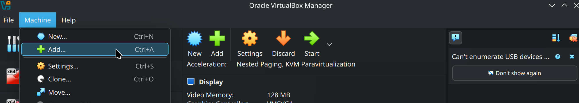
Then, you can run it by either clicking Start or simply double-clicking the virtual machine in the sidebar.
Inside the VM
If everything went well, after launching the image you should see Ubuntu’s splash screen and be dropped into the desktop directly. Below are some important things about the guest OS running on the VM.
- The VM runs Ubuntu 20.04 LTS. Any kind of “system/program error” reported by Ubuntu can safely be dismissed or ignored.
- The user on the VM is called dynamatic. The password is also dynamatic.
- On the left bar you have icons corresponding to a file explorer, a terminal, a web browser (Firefox).
- There are a couple default Ubuntu settings you may want to modify for your convenience. You can open Ubuntu settings by clicking the three icons at the top right of the Ubuntu desktop and then selecting Settings.
- You can change the default display resolution (1920x1080) by clicking on the Displays tab on the left, then selecting another resolution in the Resolution dropdown menu.
- You can change the default keyboard layout (English US) by clicking on the Keyboard tab on the left. Next, click on the + button under Input Sources, then, in the pop-menu that appears, click on the three vertical dots icon, scroll down the list, and click Other. Find your keyboard layout in the list and double-click it to add it to the list of input sources. Finally, drag your newly added keyboard layout above English (US) to start using it.
- When running commands for Dynamatic from the terminal, make sure you first
cdto thedynamaticsubfolder.- Since the user is also called dynamatic,
pwdshould display/home/dynamatic/dynamaticwhen you are in the correct folder.
- Since the user is also called dynamatic,
Advanced Build Instructions
Table of contents
- Gurobi
- Cloning
- Building
- Interactive Visualizer
- Enabling XLS Integration
- Modelsim/Questa sim installation
note
This document contains advanced build instructions targeted at users who would like to modify Dynamatic’s build process and/or use the interactive dataflow circuit visualizer. For basic setup instructions, see the installation page.
1. Gurobi
Why Do We Need Gurobi?
Currently, Dynamatic relies on Gurobi to solve performance-related optimization problems (MILP). Dynamatic is still functional without Gurobi, but the resulting circuits often fail to achieve acceptable performance.
Download Gurobi
Gurobi is available for Linux here (log in required). The resulting downloaded file will be gurobiXX.X.X_linux64.tar.gz
Obtain a License
Free academic licenses for Gurobi are available here.
Installation
To install Gurobi, first extract your downloaded file to your desired installation directory. We recommend to place this in /opt/, e.g. /opt/gurobiXXXX/linux64/ (with XXXX as the downloaded version). If extraction fails, try with sudo.
Use the following command to pass your obtained license to Gurobi, which it stores in ~/gurobi.lic
# Replace x's with obtained license
/opt/gurobiXXXX/linux64/bin/grbgetkey xxxxxxxx-xxxx-xxxx-xxxx-xxxxxxxxxxxx
note
If you chose a web library (WLS license), copy the gurobi.lic file provided to your home directory rather than running the command above
Configuring Your Environment
In addition to adding Gurobi to your path, Dynamatic’s CMake requires the GUROBI_HOME environment variable to find headers and libraries. These lines can be added to your shell initiation script, e.g. ~/.bashrc or ~/.zshrc, or used with any other environment setup method.
# Replace "gurobiXXXX" with the correct version
export GUROBI_HOME="/opt/gurobiXXXX/linux64"
export PATH="${GUROBI_HOME}/bin:${PATH}"
export LD_LIBRARY_PATH="${GUROBI_HOME}/lib:$LD_LIBRARY_PATH"
Once Gurobi is set up, you can change the buffer placement algorithm using the --buffer-algorithm compile flag and setting the value to either fpga20 or fpl22. See Using Dynamatic page for details on how to use Dynamatic and modify the compile flags.
2. Cloning
The repository is set up so that LLVM is shallow cloned by default, meaning the clone command downloads just enough of them to check out currently specified commits. If you wish to work with the full history of these repositories, you can manually unshallow them after cloning.
For LLVM:
cd dynamatic/llvm-project
git fetch --unshallow
3. Building
This section provides some insights into our custom build script, build.sh, located in the repository’s top-level folder. The script recognizes a number of flags and arguments that allow you to customize the build process to your needs. The –help flag makes the script print the entire list of available flags/arguments and exit.
note
The script should always be ran from Dynamatic’s top-level folder.
General Behavior
The build script successively builds all parts of the project using CMake and Ninja. In order, it builds
- LLVM (with MLIR and clang as additional tools),
- Dynamatic, and
- (optionally) the interactive dataflow circuit visualizer (see instructions below).
It creates build folders in the top level directory and in each submodule to run the build tasks from. All files generated during build (libraries, executable binaries, intermediate compilation files) are placed in these folders, which the repository is configured to not track. Additionally, the build script creates a bin folder in the top-level directory that contains symbolic links to a number of executable binaries built by the superproject and subprojects that Dynamatic users may especially care about.
Debug or Release Mode
The build script builds the entire project in Debug mode by default, which enables assertions in the code and gives you access to runtime debug information that is very useful when working on Dynamatic’s code. However, Debug mode increases build time and (especially) build size (the project takes around 60GB once fully built). If you do not care for runtime debug information and/or want Dynamatic to have a smaller footprint on your disk, you can instead build Dynamatic in Release mode by using the --release flag when running the build script.
# Build Dynamatic in Debug mode
./build.sh
# Build Dynamatic in Release mode
./build.sh --release
Multi-Threaded Builds
By default, Ninja builds the project by concurrently using at most one thread per logical core on your machine. This can put a lot of strain on your system’s CPU and RAM, preventing you from using other applications smoothly. You can customize the maximum number of concurrent threads that are used to build the project using the –threads argument.
# Build using at most one thread per logical core on your machine
./build.sh
# Build using at most 4 concurrent threads
./build.sh --threads 4
It is also common to run out of RAM especially during linking of LLVM/MLIR. If this is a problem, consider limiting the maximum number of parallel LLVM link jobs to one per 15GB of available RAM, using the –llvm-parallel-link-jobs flag:
# Perform at most 1 concurrent LLVM link jobs
./build.sh --llvm-parallel-link-jobs 1
note
This flag defaults to a value of 2
Dockerfile
Dynamatic includes a Dockerfile that configures all the open-source dependencies. To build the dockerfile, run the following command in the root directory of Dynamatic:
$ docker build -t dynamatic-image . --build-arg UID=$(id -u) --build-arg GID=$(id -g)
To launch the Docker container, run the following command in the root directory of dynamatic:
$ docker run -it -u $(id -u):$(id -g) -v "$(pwd):/home/ubuntu/dynamatic" -w "/home/ubuntu/dynamatic" dynamatic-image /bin/bash
which will launch the Docker container and mount the current dynamatic directory in /home/ubuntu/dynamatic.
Then you can proceed with building and running Dynamatic, for example:
$ cd /home/ubuntu/dynamatic
# Build Dynamatic using the prebuilt LLVM and enable CBC-related features.
$ bash build.sh --use-prebuilt-llvm --enable-cbc
note
We mount Dynamatic in the container since if we build it inside the docker image, it losses the states after shutting down.
Forcing CMake Re-Configuration
To reduce the build script’s execution time when re-building the project regularly (which happens during active development), the script does not try to fully reconfigure each submodule or the superproject using CMake if it sees that a CMake cache is already present on your filesystem for each part. This can cause problems if you suddenly decide to change build flags that affect the CMake configuration (e.g., when going from a Debug build to a Release build) as the CMake configuration will not take into account the new configuration. Whenever that happens (or whenever in doubt), provide the --force flag to force the build script to re-configure each part of the project using CMake.
# Force re-configuration of every submodule and the superproject
./build.sh --force
tip
If the CMake configuration of each submodule and of the superproject has not changed since the last build script’s invocation and the –force flag is provided, the script will just take around half a minute more to run than normal but will not fully re-build everything. Therefore it is safe and not too inconvenient to specify the --force flag on every invocation of the script.
Enable Cbc MILP Solver
If you have difficulty installing the Gurobi solver or getting a license, you may use the open-source alternative Cbc solver instead:
sudo apt-get install coinor-cbc
# Build Dynamatic with Cbc enabled.
./build.sh --enable-cbc
Enable Legacy Chisel-Based LSQ Generator
Dynamatic previously uses RTL generators written in Chisel (a hardware construction language embedded in the high-level programming language Scala) to produce synthesizable RTL designs. You can install JDK and Scala using the recommended way with the following commands:
sudo apt-get install -y openjdk-21-jdk
curl -fL https://github.com/coursier/coursier/releases/latest/download/cs-x86_64-pc-linux.gz | gzip -d > cs && chmod +x cs && ./cs setup
To build dynamatic with legacy LSQ enabled, append the following flag when
calling the build.sh script:
./build.sh --build-legacy-lsq
4. Interactive Dataflow Circuit Visualizer
The repository contains an optionally built tool that allows you to visualize the dataflow circuits produced by Dynamatic and interact with them as they are simulated on test inputs. This is a very useful tool for debugging and for better understanding dataflow circuits in general. It is built on top of the open-source Godot game engine and of its C++ bindings, the latter of which Dynamatic depends on as a submodule rooted at visual-dataflow/godot-cpp (relative to Dynamatic’s top-level folder). To build and/or modify this tool (which is only supported on Linux at this point), one must therefore download the Godot engine (a single executable file) from the Internet manually.
note
Godot’s C++ bindings only work for a specific major/minor version of the engine. This version is specified in the branch field of the submodule’s declaration in .gitmodules. The version of the engine you download must therefore match the bindings currently tracked by Dynamatic. You can download any version of Godot from the official archive.
Due to these extra dependencies, building this tool is opt-in, meaning that
- by default it is not built along the rest of Dynamatic.
- the CMakeLists.txt file in visual-dataflow/ is meant to be configured independently from the one located one folder above it i.e., at the project’s root. As a consequence, intermediate build files for the tool are dumped into the
visual-dataflow/build/folder instead of the top-levelbuild/folder.
Building an executable binary for the interactive dataflow circuit visualizer is a two-step process, one which is automated and one which still requires some manual work detailed below.
- Build the C++ shared library that the Godot project uses to get access to Dynamatic’s API. The
--visual-dataflowbuild script flag performs this task automatically.
# Build the C++ library needed by the dataflow visualizer along the rest of Dynamatic
./build.sh --visual-dataflow
At this point, it becomes possible to open the Godot project (in the /dynamatic/visual-dataflow directory) in the Godot editor and modify/run it from there. Run your downloaded Godot file and open the project in the visual data-flow directory.
- export the Godot project as an executable binary to be able to run it from outside the editor. In addition to having downloaded the Godot engine, at the moment this also requires that the project has been exported manually once from the Godot editor. The Godot documentation details the process here, which you only need to follow up to and including the part where it asks you to download export templates using the graphical interface. Once they are downloaded for your specific export target, you are now able to automatically build the tool by using the
--export-godotbuild script argument and specifying the path to the Godot engine executable you downloaded.
Quick Steps From Godot Tutorial
- Download Godot
- Build Dynamatic with
--visual-dataflowflag - Run Godot (from the directory to which it was downloaded)
- Click
Editorin the top navigation bar and selectManage Export Templates - Click
Onlinebutton, download and Install Export Templates - Click
Projectbutton at top left of editor and select Export - Click the
Export PCK/ZIP...enter a name for your export and validate it
For more details, visit official godot engine website.
Finally, run the command below to export the Godot project as an executable binary that will be accessed by Dynamatic
# Export the Godot project as an executable binary
# Here it is a good idea to also provide the --visual-dataflow flag to ensure
# that the C++ library needed by the dataflow visualizer is up-to-date
./build.sh --visual-dataflow --export-godot /path/to/godot-engine
The tool’s binary is generated at visual-dataflow/bin/visual-dataflow and sym-linked at bin/visual-dataflow for convenience.
Now, you can visualize the dataflow graphs for your compiled programs with Godot. See how to use Dynamatic for more details.
note
Whenever you make a modification to the C++ library or to the Godot project itself, you can simply re-run the above command to recompile everything and re-generate the executable binary for the tool.
5. Enabling the XLS Integration
The experimental integration with the XLS HLS tool (see here for more information) can be enabled by providing the --experimental-enable-xls flag to build.sh.
note
--experimental-enable-xls, just like any other cmake-related flags, will only be applied if ./build.sh configures CMake, which it, by default, will not do if a build folder (with a CMakeCache.txt) exists. To enable xls if you already have a local build, you can either force a reconfigure of all projects by providing the --force flag, or delete the Dynamatic’s CMakeCache.txt to only force a reconfigure (and costly rebuild) of Dynamatic:
./build.sh --force --experimental-enable-xls
# OR
rm build/CMakeCache.txt
./build.sh --experimental-enable-xls
Once enabled, you do not need to provide ./build.sh with --experimental-enable-xls to re-build.
6. Modelsim/Questa Installation
Dynamatic uses Modelsim (has 32 bit dependencies) or Questa (64 bit simulator) to run simulations, thus you need to install it before hand. Download Modelsim or Questa, install it (in a directory with no special access permissions) and add it to path for Dynamatic to be able to run it. Add the following lines to the .bashrc file in your home directory to add modelsim to path variables.
note
Ensure you write the full path
export MODELSIM_HOME=/path/to/modelsim  # path will look like /home/username/intelFPGA/20.1/modelsim_ase
export PATH="$MODELSIM_HOME/bin:$PATH"  # (adjust the path accordingly)
or
export MODELSIM_HOME=/path/to/questa    # path will look like home/username/altera/24.1std/questa_fse/
export PATH="$MODELSIM_HOME/bin:$PATH"
In any terminal, source .bashrc file and run the vsim command to verify that modelsim was added to path properly and runs.
source ~/.bashrc
vsim
If you encounter any issue related to libXext (if you installed Modelsim) you may need to install a few more libraries to enable the 32 bit architecture which supports packages needed by Modelsim:
sudo dpkg -add-architecture i386
sudo apt update
sudo apt install libxext6:i386 libxft2:i386 libxrender1:i386
If you are using Questa, running vsim will give you an error relating to the absence of a license.
To obtain a license (free or paid):
- Create an account on Intel’s Self Servicing License Center page. The page has detailed instructions on how to obtain a license.
- Request for a license. You will receive an authorization email with instructions on setting up a fixed or floating license (a fixed license suffices). This could take some minutes or up to a few hours.
- Download the license file and add it to path as shown below
#Questa license set up
export LM_LICENSE_FILE=/path/to/license/file     # looks like this "home/username/.../LR-240645_License.dat:$LM_LICENSE_FILE"
export MGLS_LICENSE_FILE=/path/to/license/file   # looks like this "/home/beta-tester/Downloads/LR-240645_License.dat"
export SALT_LICENSE_SERVER=/path/to/license/file # looks like this "/home/beta-tester/Downloads/LR-240645_License.dat"
note
You may need only one of the three lines above based on the version of Questa you are using. Refer to the release notes for the version you have installed. Having the three lines poses no issue nonetheless.
Analyzing Output Files
Dynamatic stores the compiled IR, generated RTL, simulation results, and useful intermediate data in the out/ directory.
Learning about these files is essential for identifying performance bottlenecks, gaining deeper insight into the generated circuits, exporting the generated design to integrate into your existing designs, etc.
This document provides guidance on the locations of these files and how to analyze them effectively.
Compilation Results
note
Compilation results are not essential for a user but can help in debugging. This requires some knowledge of MLIR.
- The
compilecommand creates anout/compdirectory that stores all the intermediate files as described in the Dynamatic HLS flow in the developer guide. - A file is created for every step of the compilation process, allowing the user to inspect relevant files if any unexpected behaviour results.
tip
Compilation results in the creation of two PNG file, kernel_name.png and kernel_name_CFG.png, allowing the user to have an overview of the generated circuit and associated control flow graph of their kernel.
RTL Generation Results
The write-hdl command creates an out/hdl directory.
out/hdl contains all the RTL files (adders, multipliers, muxes, etc.) needed to implement the target kernel.
The top level HDL file is called kernel_name.vhd or kernel_name.v if you use VHDL or verilog respectively.
Simulation Results
important
Modelsim/Questa must be installed and added to path before running this command. See Modelsim/Questa installation guide
The simulate command creates an out/sim directory. In this directory are a number of sub directories organized as shown below:
out/sim
├── C_OUT           # output from running the C program
├── C_SRC           # C source files and header files
├── HDL_OUT         # output from running the simulation of the HDL testbench
├── HDL_SRC         # HDL files and the testbench
├── HLS_VERIFY      # Modelsim/Questa files used to run simulation
├── INPUT_VECTORS   # inputs passed to the C and HDL implementations for testing
├── report.txt      # simulation report and logs
The simulate command runs a C/HDL co-simulation and prints the SUCCESS message when the results are the same. The comments next to each directory above give an overview of what they contain.
note
The report.txt is of special interest as it gives the user information on the simulation in both success and failure situations. If successful, the user will get information on runtime and cycle count. Otherwise, information on the cause of the failure will be reported.
tip
The vsim.wlf file in the HLS_VERIFY directory contains information on simulation, the different signals and their transitions over time.
Visualization Results
important
Dynamatic must have been build with Godot installed and the --visual-dataflow flag to use this feature. See interactive visualizer setup
The visualize command creates an out/visual directory where a LOG file is generated from the Modelsim/Questa wlf file created during simulation. he LOG file is converted to CSV and visualized using the Godot game engine, alongside the DOT file that represents the circuit structure.
Vivado Synthesis Results
important
Vivado must be installed and sourced before running this command
The synthesize command creates an out/synth directory where timing and resource information is logged. Users can view information on:
- clock period and timing violations
- resource utilization
- report on vivado synthesis
The file names are intuitive and would allow users to find the information they need
Command Reference
The Dynamatic shell is an interactive command line-based interface (you can launch it from Dynamatic’s top level directory with ./bin/dynamatic after building Dynamatic) that allows users to interact with Dynamatic and use the different commands available to generate dataflow circuits from C code.
This document provides an overview of the different commands available in the Dynamatic frontend and their respective flags and options.
Dynamatic Shell Commands
help: Display list of commands.set-dynamatic-path <path>: Set the path of the root (top-level) directory of Dynamatic, so that it can locate various scripts it needs to function. This is not necessary if you run Dynamatic from said directory.set-vivado-path <path>: Set the path to the installation directory of Vivado.set-polygeist-path <path>: Sets the path to the Polygeist installation directory.set-fp-units-generator <flopoco|vivado>: Choose which floating point unit generator to use. See this section for more information.set-clock-period <clk>: Sets the target clock period in nanoseconds.set-src <source-path>: Sets the path of the.cfile of the kernel that you want to compile.compile [...]: Compiles the source kernel (chosen byset-src) into a dataflow circuit. For more options, runcompile --help.
note
The compile command does not require Gurobi by default, but it is needed for smart buffer placement options.
The --buffer-algorithm flag allows users to use smart buffer placement algorithms notably fpga20 and fpl22 for throughput and timing optimizations.
The --fast-token-delivery flag enables the Fast Token Delivery (FTD) algorithm during the CF → Handshake lowering stage. Note that this option is currently incompatible with smart buffer placement algorithms.
write-hdl [--hdl <vhdl|verilog|smv>]: Convert results fromcompileto a VHDL, Verilog or SMV file.simulate [--simulator <vsim|xsim|ghdl|verilator]: Simulates the HDL produced bywrite-hdl.
note
Requires a ModelSim/Questa (vsim), Vivado (xsim), GHDL (ghdl) or Verilator (verilator) installation.
synthesize: Synthesizes the HDL result fromwrite-hdlusing Vivado.
note
Requires a Vivado installation!
verify-invariants: Verify that automatically-generated invariants during rigidification are provably correct.
note
Requires nuXmv installation!
visualize: Visualizes the execution of the simulated circuit.
note
Requires Godot Engine and the visualizer component must be built!
exit: Exits the interactive Dynamatic shell.
For more information and examples on the typical usage of the commands, checkout the using Dynamatic and example pages.
Dependencies
Dynamatic uses a number of libraries and tools to implement its full functionality. This document provides a list of these dependencies with some information on them.
Libraries
Git Submodules
Dynamatic uses git submodules to manage its software dependencies (all hosted on GitHub). We depend on Polygeist, a C/C++ frontend for MLIR which itself depends on LLVM/MLIR through a git submodule. The project is set up so that you can include LLVM/MLIR headers directly from Dynamatic code without having to specify their path through Polygeist. We also depend on godot-cpp, the official C++ bindings for the Godot game engine which we use as the frontend to our interactive dataflow circuit visualizer. See the git submodules guide for a summary on how to work with submodules in this project.
Polygeist
Polygeist is a C/C++ frontend for MLIR including polyhedral optimizations and parallel optimizations features. Polygeist is thus responsible for the first step of our compilation process, that is taking source code written in C/C++ into the MLIR ecosystem. In particular, we care that our entry point to MLIR is at a very high semantic level, namely, at a level where polyhedral analysis is possible. The latter allows us to easily identify dependencies between memory accesses in source programs in a very accurate manner, which is key to optimizing the allocation of memory interfaces and resources in our elastic circuits down the line. Polygeist is able to emit MLIR code in the Affine dialect, which is perfectly suited for this kind of analysis.
CMake & Ninja
These constitute the primary build system for Dynamatic. They are used to build Dynamatic core, Polygeist, and LLVM/MLIR. You can have more details on CMake and Ninja by checking their official documentations.
Boost.Regex
Boost.Regex is used to resolve Dynamatic regex expressions.
Scripting & Tools
Python (≥ 3.6)
Used in build systems, scripting, testing. See official documentation
Graphviz (dot)
Generates visual representations of dataflow circuits (i.e., .dot). See official documentation
JDK (Java Development Kit)
Required to run Scala/Chisel compilation. See official documentation.
Tools
Dynamatic uses some third party tools to implement smart buffer placement, simulation, and interactive dataflow circuit visualization. Below is a list of the tools:
Optimization & Scheduling: Gurobi
Gurobi solves MILP (Mixed-Integer Linear Programming) problems used during buffer placement and optimization. Dynamatic is still functional without Gurobi, but the resulting circuits often fail to achieve acceptable performance. See how to set up gurobi in the advanced build section
Simulation Tool: ModelSim/Questa
Dynamatic uses ModelSim/Questa to perform simulations. See installation page on how to setup ModelSim/Questa.
Graphical Tools: Godot
godot-cpp, the official C++ bindings for the Godot game engine which we use as the frontend to our interactive dataflow circuit visualizer.
Utility/Development Tools
clang, lld, ccache
These are optional compiler/linker improvements to speed up builds. See their official documentations for details.
Git
Dynamatic uses git for project and submodule version control
Standard UNIX Toolchain: curl, gzip, etc.
These are used for the various build scripts in the Dynamatic project.
Writing Hls C Code for Dynamatic
Before passing your C kernel (function) to Dynamatic for compilation, it is important that you ensure it meets some guidelines. This document presents the said guidelines and some constraints that the user must follow to make their code suitable inputs for Dynamatic.
note
These guidelines target the function to be compiled and not the main function of your program except for the CALL_KERNEL. Main is primarily useful for passing inputs for simulation and is not compiled by Dynamatic
Summary
- Dynamatic header
CALL_KERNELmacro inmain- Variable Types and Names in
mainMust Match Parameter Names in Kernel Declaration - Inline functions called by the kernel
- No recursive calls
- No pointers
- No dynamic memory allocation
- Pass global variables
- No support for local array declarations
- Data type support
1. Include the Dynamatic Integration Header
To be able to compile in Dynamatic, your C files should include the Integration.h header that will be a starting point for accessing other relevant Dynamatic libraries at compile time.
#include "dynamatic/Integration.h"
2. Use the CALL_KERNEL Macro in the main Function
Do not call the kernel function directly, use the CALL_KERNEL macro provided through Dynamatic’s integration header.
It does two things in the compiler flow:
- Dumps the argument passed to the kernel to files in sim/INPUT_VECTORS (for C/HDL cosimulation when the
simulatecommand is ran). - Dumps the argument passed to the kernel to a profiler to determine which loops are more important to be optimized using buffer placement.
CALL_KERNEL(func, input_1, input_2, ... , input_n)
3. Match Variable Names and Types in main to the Parameter Declared as Kernel Inputs
For simulation purposes, the variables declared in the main function must have the same names and data types as the function parameters of your function under test. This makes it easy for the simulator to correctly identify and properly match parameters when passing them. For example:
void loop_scaler(int arr[10], int scale_factor){
    ...
}; // function declaration

int main(){
    int arr[10]; // same name and type
    int size;    // as in kernel declaration

    scale_factor = 50;
    // initialize arr[10] values

    CALL_KERNEL(loop_scaler, arr, scale_factor);
    return 0;
}
Limitations
1. Do Not Call Functions in Your Target Function
The target function is the top level function to be implemented by Dynamatic. Dynamatic does not support calling other functions in the target kernel. Alternatively, you can use macros to implement any extra functionality before using them in your target kernel.
#define increment(x) x+1; // macro for increment function

void loop(int x) {
    while (x<20) {
        increment(x); // macro
    }
}  // inlined with macro definition.
2. Recursive Calls Are Not Supported
Like other HLS tools, Dynamatic does not support recursive function calls because:
- they are difficult to map to hardware
- have unpredictable depths and control flow
- unbounded execution
- the absence of call-stack in FPGA platforms would be too resource demanding to implement efficiently epecially without knowing the bounds ahead of time.
An alternative would be to manually unroll recursive calls and replace them with loops where possible.
3. Pointers Are Not Supported
Pointers should not be used. *(x + 1) = 4; is invalid. Use regular indexing and fixed sized arrays if need be as shown below.
int x[10]; // fixed sized
x[1] = 4; // non-pointer indexing
4. Dynamic Memory Allocation is Not Supported
Dynamic memory allocation is also not allowed because it’s not deterministic enough to allow enough hardware resources to be allocated at compile time.
5. Global Variables
Dynamatic compiles the kernel code only. Any variables declared outside the kernel function will not be converted unless they are passed to the kernel. Global variables are no exception. You can pass global variables as parameters to your kernel or define them as macros to make your kernel simpler.
#define scale_alternative (2)
int scale = 2;

int scaler(int scale, int number) // scale is still passed as parameter
{
    return number * scale * scale_alternative;
}
6. Local Array Declarations are Not Supported
Local array declaration in kernels is not yet supported by Dynamatic. Pass all arrays as parameters to your kernel.
void convolution(unsigned char input[HEIGHT][WIDTH], unsigned char output[HEIGHT][WIDTH]) {

    int kernel[3][3] = {
        {1, 1, 1},
        {1, 1, 1},
        {1, 1, 1}
    };
    int kernel_sum = 9;

    for (int y = 1; y < HEIGHT - 1; y++) {
        for (int x = 1; x < WIDTH - 1; x++) {
            int sum = 0;
            for (int ky = -1; ky <= 1; ky++) {
                for (int kx = -1; kx <= 1; kx++) {
                    sum += input[y + ky][x + kx] * kernel[ky + 1][kx + 1]; // one issue hear...non-affine apparently..
                                                                        // the kernel indexing is considered non-affine
                }
            }
            output[y][x] = sum / kernel_sum;
            printf("output[%d][%d] = %d\n", y, x, output[y][x]);
        }
    }
}
The above code will yield an error at compilation about array flattening. Pass it as a parameter to bypass the error:
void convolution(int kernel[3][3], unsigned char input[HEIGHT][WIDTH], unsigned char output[HEIGHT][WIDTH])
Data Types Supported by Dynamatic
These types are most crucial when dealing with function parameters. Some of the unsupported types may work on local variables without any compilation errors.
note
Arrays of supported data types are also supported as function parameters
| Data type | Supported |
|---|---|
| unsigned | ✓ |
| int32_t / int16_t / int8_t | ✓ |
| uint32_t / uint16_t / uint8_t | ✓ |
| char / unsigned char | ✓ |
| short | ✓ |
| float | ✓ |
| double | ✓ |
| _BitInt(N) | ✓ |
| long/long long/long double | x |
| uint64_t / int64_t | x |
| __int128 | x |
note
The _BitInt(N) is a bit-percise integer type introduced in C23. We can use
it to represent integers with arbitrary width, e.g., a 18-bit integer.
Example:
_BitInt(7) foo = 3;
signed _BitInt(19) bar = -17;
Dynamatic support this datatype in both synthesis and C-to-RTL co-simulation.
Supported Operations
- Arithmetic operations:
+,-,*,/,++,--. - Logical operations on
int:>,<,&&,||,!,^
Unsupported Operations
- Arithmetic operations:
% - Pointer operations:
*,&(indexing is supported -a[i]) - Most math functions excluding absolute value functions
- Logical operations can be used with variables of type
floatin C but the following are not yet supported in Dynamatic:&&,||,!,^.
tip
Data type and operation related errors generally state explicitly that an operation or type is not supported. Kindly report those as bugs on our repository while we work on making more data types supported.
Other C Constructs
Structs
structs are currently not supported. Consider passing inputs individually rather than grouping with structs
Function Inlining
The inline keyword is not yet supported. Consider #define as an alternative for inlining blocks of code into your target function
Volatile
The volatile keyword is supported but has zero impact on the circuits generated.
warning
Do not use on function parameters!
Dynamatic is being refined over time and is yet to support certain constructs such as local array declarations in the target function which must rather be passed as inputs. If you encounter any issue in using Dynamatic, kindly report the bug on the github repository.
In the meantime, visit our examples page to see an example of using Dynamatic.
Optimizations And Directives
Dynamatic offers a number of options to optimize the generated RTL code to meet specific requirements. This document describes the various optimization options available as well as some directives to customize the generated RTL to specific hardware using proprietory floating point unit generators.
Overview: What if I Want to Optimize …
- Clock frequency
- Area
- Latency and throughput
- Customizing Design to Specific Hardware: Floating Point IPs
- Optimization algorithms in Dynamatic
- Custom compilation flows
1. Achieving a Specific Clock Frequency
Dynamatic relies on its buffer placement algorithm to regulate the critical path in the design to achieve a specific frequency target. To achieve the desired target, set the period (set-clock period <value_in_ns>) and enable the buffer placement algorithm compile --buffer-algorithm <...>...
2. Area
Circuit area can be optimized using the following compile flags
- LSQ sizing
- Credit-based resource sharing:
--sharing - Buffer placement :
--buffer-algorithmwith valuefpl22
3. Latency and Throughput
Latency and throughput can be improved using buffer placement with either the fpga20 or fpl22 values for the --buffer-algorithm compile flag.
Adjusting Design to Specific Hardware: Floating Point IPs
Dynamatic uses open-source FloPoCo components proprietory Vivado to allow users to customize their floating point units. For instructions on how to achieve this, see the floating point units guide. Floating point units can be selected using the set-fp-units-generator <flopoco|vivado> command as shown in the command reference.
Advantages of Using Vivado Over FloPoCo Floating Point IP
- Tailored for Xilinx hardware and ideal for industry level projects.
- Supports IEEE-754 single, double, and half precision floating point representation.
- Supports NaN, infinity, denormals, exception flags, and rounding models.
- Provides plug and play floating point units.
Advantages of Using FloPoCo Over Vivado Floating Point IP
- Open source, hence ideal for academic research involving fine grained parameter tuning and RTL transparency
- Very good for custom floating point formats such as FP8 or “quasi-floating point”.
- Users can explicitly control pipeline depth.
- Generated RTL is portable to any toolchanin unlike Vivado which is limited to Xilinx-specific resources.
Optimization Algorithms in Dynamatic
Throughput Optimization: Enabling Smart Buffer Placement
Dynamatic automatically inserts buffers to eliminate performance bottlenecks and achieve a particular clock frequency. This feature is essential to enable for Dynamatic to achieve the best performance.
For example, the code below:
int fir(in_int_t di[N], in_int_t idx[N]) {
  int tmp = 0;
  for (unsigned i = 0; i < N; i++)
    tmp += idx[i] * di[N_DEC - i];
  return tmp;
}
has a long latency multiplication operation, which prolongs the lifetime of loop variables. Buffers must be sufficiently and appropriately inserted to achieve a certain initiation interval.
The naive buffer placement (default) algorithm in Dynamatic, on-merges, is used by default. Its strategy is to place buffers on the output channels of all merge-like operations. This creates perfectly valid circuits, but results in poor performance.
For better performance, two more advanced algorithms are implemented, based on the FPGA’20 and FPL’22 papers. They can be chosen by using compile in bin/dynamatic with the command line option --buffer-algorithm fpga20 or --buffer-algorithm fpl22, respectively.
note
These two algorithms require Gurobi to be installed and detected, otherwise they will not be available!
Installation instructions for Gurobi can be found here. A brief high-level overview of these algorithms’ strategies is provided below; for more details, see the original publications linked above and this document.
Buffer Placement Algorithm: FPGA’20
The main idea of the fpga20 algorithm is to decompose the dataflow circuit into choice-free dataflow circuits (i.e. parts which don’t contain any branches). The performance of these CFDFCs can be modeled using an approach based on timed Petri nets (see Performance Evaluation of Asynchronous Concurrent Systems Using Petri Nets and Analysis of asynchronous concurrent systems by timed petri nets).
This model is formulated as a mixed-integer linear programming model (MILP), with additional constraints which allow the optimization of multiple CFDFCs. Simulation results have shown circut speedups up to 10x for most benchmarks, with some reaching even 33x. For example, the fir benchmark with naive buffering runs in 25.8 us, but with this algorithm, it executes in only 4.0 us, which is 6.5x faster.
The downside is that the MILP solver can take a long time to complete its task, sometimes even more than an hour, and also clock period targets might not be met.
Buffer Placement Algorithm: FPL’22
The fpl22 algorithm also uses a MILP-based approach for modeling and optimization. The main difference is that it does not only model the circuit as single dataflow channels carrying tokens, but instead, describes individual edges carrying data, valid and ready signals, while explicitly indicating their interconnections. The dataflow units themselves are modeled with more detail. Instead of nodes representing entire dataflow units, they represent distinct combinational delays of every combinational path through the dataflow units. This allows for precise computation of all combinational delays and accurate buffer placement for breaking up long combinational paths.
This approach meets the clock period target much more consistently than the previous two approaches.
Area Optimization: Sizing Load-Store Queue Depths: FPT’22
In order to leverage the power of dataflow circuits generated by Dynamatic, a memory interface is required which would analyze data dependencies, reorder memory accesses and stall in case of data hazards. Such a component is a Load-Store Queue, specifically designed for dataflow circuits. The LSQ sizing algorithm is implemented based on FPT’22
The strategy for managing memory accesses is based on the concept of groups.
note
A group is a sequence of memory accesses that cannot be interrupted by a control flow decision.
Determining a correct order of accesses within a group can be done easily using static analysis and can be encoded into the LSQ at compile time. The LSQ component has as many load/store ports as there are load/store operations in the program. These ports are clustered by groups, with every port belonging to one group. Whenever a group is “activated”, all load/store operations belonging to that group are allocated in the LSQ in the sequence that was determined by static analysis. Once a group has been allocated, the LSQ expects each of the corresponding ports to eventually get an access; dependencies will be resolved based on the order of entries in the LSQ.
warning
A significant area improvement can be achieved by disabling the use of LSQs but this must be used cautiously.
The specifics of LSQ implementation are available in the corresponding documentation. For more information on the concept itself, see the original paper.
Resource Sharing of Functional Units: ASPLOS’25
Dynamatic uses a resource sharing strategy based on ASPLOS’25. This algorithm avoids sharing-introduced deadlocks by decoupling interactions of operations in shared resources to break resource dependencies while maintaining the benefits of dynamism. It is activated using the --sharing compile flag as such:
compile <...> --sharing
Handshake Logic Optimization via Rigidification
Dynamatic uses formal verification to prove handshake logic redundancy (described in FPGA’23), the proven redundancy can be safely removed without penalizing the performance.
To enable this feature in Dynamatic, we need to pass an additional argument to build.sh.
# Downloads the model checker and enable test cases in CI/CD pipeline.
bash build.sh --enable-leq-binaries
This makes the rigidification optimization feature available in the CLI tool bin/dynamatic. To enable this feature in an HLS flow, we can pass an additional argument to the compile CLI command:
# Generate formal model in the nuXmv input language (.smv), prove logic redundancy properties, and produce a
# circuit with simplified handshake logic.
compile <...> --rigidification
Custom Compilation Flows
Some other transformations also optimize the circuit, but they are not included in the normal compilation flow.
In such case, one should invoke components such as dynamatic-opt (also located in the bin directory) directly. The default compilation flow is implemented in tools/dynamatic/scripts/compile.sh; you can use this as a template that you can adjust to your needs.
Some optimization strategies, such as speculation or fast token delivery, aren’t accessible through the standard dynamatic interactive environment.
These approaches often require a custom compilation flow. For example, speculation provides a Python script that enables a push-button flow execution.
For more details, refer to the speculation documentation.
LSQ
If the Dynamatic compiler cannot statically disambiguate memory accesses, it will instantiate spatial load-store queues (LSQs). They sit between elastic datapath and memory array and are responsible for ordering memory accesses (i.e., loads and stores) sufficiently to guarantee program correctness. If possible, they allow out-of-order execution of memory accesses to improve kernel performance by delivering load data to the datapath as quickly as possible.
Example
Consider this histogram kernel as a simple example:
void histogram(int[] hist, int[] idx, int n) {
  for (int i = 0; i < n ; i++)
    hist[idx[i]] += 1;
}
Each iteration of this kernel increments some entry of the hist array.
However, which entry is modified is not known statically, since it depends on the idx array, which is itself an input to the kernel.
This necessitates use of an LSQ to ensure correctness.
The simplest possible LSQ would simply enforce that all memory accesses to the hist array are performed in program order, as shown here:
LD hist[idx[0]]ST hist[idx[0]]LD hist[idx[1]]ST hist[idx[1]]- and so on… This would guarantee correctness, but sacrifices substantial performance. The reason is that the in-order execution of memory accesses effectively means that consecutive loop iterations do not overlap (or rather, overlap very little). Put differently, the loop initiation interval (II) is approximately the latency of the load-increment-store path.
Now consider the best case, where all idx values are different.
In that case, an ideal schedule would simply use an II of 1:
there is no need to order memory accesses from one loop iteration with respect to another loop iteration.
Clearly, executing memory accesses out-of-order can increase performance substantially.
This potential is realized by using more complex out-of-order spatial LSQs.
Out-of-Order LSQs
Dynamatic’s spatial LSQ is based on a design described in this TECS’17 paper.
Overview
The LSQ uses two circular queue structures to hold load and store requests, respectively. Each time a basic block is entered, all its memory operations (the group) are allocated into the two queues (in-order) by the group allocator. The LSQ then interfaces with all load and store operators and accepts operands (load/store addresses and store data) out-of-order, placing them into the pre-allocated queue slots. As soon as a memory request is ready (i.e., all its operands are available), it may be executed by the out-of-order issue logic of the LSQ. For stores, the request completes with the arrival of the (empty) response from memory, and the store queue entry is deallocated. For loads, data arrives back from memory and is placed back into the queue. From there, it is returned to the circuit’s load operators, and the load queue entry is deallocated.
Out-of-Order Features
The LSQ supports out-of-order execution by comparing requests’ memory addresses at runtime: if a load and a store target different memory locations, they can (in principle) be executed out of order.
In the following, we describe the different out-of-order features supported by the LSQ and describe which workloads they benefit.
Allowing Loads to Skip Older Stores
If a load is younger than a store (i.e., the store comes first in program order) and they target different addresses, the load can safely be executed before the store.
This is the most commonly used out-of-order feature of the LSQ.
For example, it is what unlocks most performance in the above histogram example kernel, since it allows loads to “run ahead” of stores in the absence of conflicts.
Allowing Stores to Skip Older Loads
If a store is younger than a load (i.e., the load comes first in program order) and they target different addresses, the store can safely be executed before the load.
This feature is used less frequently due to the nature of most compute kernels. They typically load some data, perform some computations, and then store it at the end. For this reason, once a store’s operands are available, all previous loads have typically completed. In many cases, there is even a data dependency between these loads and the store. One (constructed) example where this might be beneficial is:
void store_before_load(int a[], int b[], int n) {
  for (int i = 0; i < n; i++) {
    int x, y;
    x = a[i]                     // load 1
    y = b[(x * x + x) / 3 + x];  // load 2
    b[x] = 1;                    // store 3
    b[x + 1] = y;                // store 4
  }
}
In this example, the index for load 2 requires a complex computation involving x, while store 3 only requires x itself and the constant 1 as its operands.
In this case, store 3 could execute ahead of load 2.
Allowing Loads to Skip Older Loads
Sometimes, the load that is “next in line” cannot be executed, either because its address is not known yet, or because the LSQ has determined that it conflicts with an older store that it needs to wait for. In these cases, the LSQ allows younger loads to “skip ahead” and execute before the older load (given they are not blocked themselves).
This feature is rarely needed in practice. However, it can significantly increase performance if address sequences have certain structures. Consider the (constructed) example:
void load_before_load(int x[], int idx1[], int idx2[], int idx3[]) {
  for (int i = 0; i < n; i++)
    int a, b;
    a = x[idx1[i]];      // load 1
    b = x[idx2[i]];      // load 2
    x[idx3[i]] = a + b;  // store 3
}
Depending on the contents of idx1, idx2, and idx3, this kernel may benefit from this feature.
If idx1[i] matches idx3[i-1], then load 1 cannot execute because it has to wait for the previous iteration’s store 3 to complete.
If idx2[i] does not have the same issue, then load 2 could execute ahead of load 1, which reduces the time until both a and b are available.
Among Dynamatic’s integration tests, this feature is most beneficial for the matrix_power kernel, which has a similar (but more complex) structure to the above example.
Allowing Stores to Skip Older Stores
If the “next in line” store cannot be executed because it is blocked (unknown address, missing data, or conflict with older load), it would be possible for a younger store to “skip ahead” and execute first. As with loads skipping ahead of older loads, the younger store would need to have its operands available. However, with stores, there is an additional condition. A store may not execute ahead of an older store with the same address (as this would constitute a write-after-write hazard).
To avoid comparing store addresses with one another, which comes with additional complexity and resource cost, Dynamatic’s LSQ does not support this feature. This means that stores (among themselves) are executed fully in program order.
We believe the benefits of this feature would be very minor for real-world workloads.
Store-to-Load Forwarding (Bypass)
If a load targets the same address as a previous store, the LSQ can bypass the store data directly to the subsequent load, given that:
- the store address is known,
- the load address is known,
- the store and load addresses are equal,
- all stores ordered between the store and the load have known addresses which are different from the load address.
With this feature, loads which conflict with earlier stores can have their load data returned earlier since it avoids the latency of two memory roundtrips (one to write, one to read back). Furthermore, the memory read can be omitted (the write operation is still needed), which saves memory read bandwidth.
Bypass is most useful for kernels with frequent conflicts, since they benefit more from the reduced latency. One such example is a naive matrix-vector multiplication kernel like this:
void matvec(int y[], int a[], int x[], int n) {
  for (int i = 0; i < n; i++) {
    y[i] = 0;
    for (int j = 0; j < n; j++) {
      y[i] += a[i * n + j] * x[j];
    }
  }
}
In this case, every load from y[i] will conflict with the previous store, so bypass would reduce the latency of each load.
However, this example is not ideal, as the accumulator could simply be stored in a temporary variable and only written to memory once at the end.
This would eliminate the need for an LSQ entirely.
Bypass is especially beneficial for workloads that are constrained by memory read bandwidth (e.g., because they perform multiple reads for each write) and have frequent conflicts (so that bypass path is used regularly). By reducing the number of reads from memory, bypass can lower the II from (for example) 2 to 1, thereby doubling throughput and approximately halving kernel latency.
Resource Cost and Timing Considerations
While out-of-order LSQs can help minimize kernel latencies, they consume significant resources and can impact the circuit’s critical path. We describe the trade-off between minimizing latency and minimizing resource cost and/or critical path below.
Note: A configuration file is used to specify LSQ parameters such as load/store queue depth and whether the bypass network is enabled. The compiler currently hard-codes the queue depths to 16 and always enables the bypass network. These parameters are currently not exposed to users of Dynamatic. However, they could be manually overridden in
dynamatic/tools/backend/lsq-generator-python/core_gen/configs.py. When doing that, care must be taken in case a kernel includes multiple LSQs. One option to expose the configuration of LSQs to the user would be through pragmas in the kernel source code.
Resource Cost
A fully-fledged out-of-order LSQ in Dynamatic can dominate total resource usage, especially when attached to small datapaths.
The main drivers of resource cost are (in this order) the bypass network and the out-of-order issue logic (including address comparators). The bypass network could be disabled completely if it is not beneficial for a given workload, saving up to half of total LSQ resources. In general, most logic scales with load/store queue depth or even with their product.
Thus, reducing queue sizes can significantly reduce total resource usage. However, this can come at a latency cost, since smaller queues fill up more quickly, which can cause backpressure into the datapath and stall the entire circuit. Nevertheless, this can be an effective lever if the LSQ’s resource cost is prohibitive otherwise. There is no potential for deadlocks or incorrect results even with very small queue depths. The only constraint is that the queues are large enough to allocate the loads/stores from each basic block at once (with one additional entry free in each queue).
Timing (Critical Path)
Next to high resource cost, the LSQ often includes long timing paths, which may be critical in the overall design. If the LSQ is responsible for the critical path, it is usually either at its output (where load data is returned to the circuit) or within the bypass network.
All these paths typically include cyclic priority masking units, whose delay is linear in either the load or store queue depth (not their product).
Working With Submodules
Having a project with submodules means that you have to pay attention to a couple additional things when pulling/pushing code to the project to maintain it in sync with the submodules. If you are unfamiliar with submodules, you can learn more about how to work with them here. Below is a very short and incomplete description of how our submodules are managed by our repository as well as a few pointers on how to perform simple git-related tasks in this context.
Along the history of Dynamatic’s (in this context, called the superproject) directory structure and file contents, the repository stores the commit hash of a specific commit for each submodule’s repository to identify the version of each subproject that the superproject currently depends on. These commit hashes are added and commited the same way as any other modification to the repository, and can thus evolve as development moves forward, allowing us to use more recent version of our submodules as they are pushed to their respective repositories. Here are a few concrete things you need to keep in mind while using the repository that may differ from the submodule-free workflow.
-
Clone the repository with
git clone --recurse-submodules git@github.com:EPFL-LAP/dynamatic.gitto instruct git to also pull and check out the version of the submodules referenced in the latest commit of Dynamatic’smainbranch. -
When pulling the latest commit(s), use
git pull --recurse-submodulesfrom the top level repository to also update the checked out commit from submodules in case the superproject changed the subprojects commits it is tracking. -
To commit changes made to files within Polygeist from the superproject (which is possible thanks to the fact that we use a fork of Polygeist), you first need to commit these changes to the Polygeist fork, and then update the Polygeist commit tracked by the superproject. More precisely,
cdto thepolygeistsubdirectory,git addyour changes andgit committhem to the Polygeist fork,cdback to the top level directory,git add polygeistto tell the superproject to track your new Polygeist commit andgit committo Dynamatic.
If you want to push these changes to remote, note that you will need to
git pushtwice, once from thepolygeistsubdirectory (the Polygeist commit) and once from the top level directory (the Dynamatic commit).
Verifying the Generated Design
Circuits generated by Dynamatic are tested against the original C implementation to ascertain their correctness using the simulate command. To gain a good understanding of the quality of the generated circuits, users can explore the files generated by this command and/or use the interactive dataflow circuit visualizer to have a more visual assessment of their circuit.
This document focuses on the content of the out/sim directory and helps the user understand the relevance of this content in assessing their circuits.
C-RTL Cosimulation
Dynamatic has a cosimulation framework that allows the user to write a testbench in C code (the main function). To take advantage of this, you must ensure that you:
- Include the
dynamatic/Integration.hheader - Create a main function where your test inputs will be instantiated
- Make a function call to the function under test in the main function using the following syntax:
CALL_KERNEL(<func_name>, <arg1>, <arg2>, ..., <argN>);. The values of the arguments passed to the function (i.e.,<arg1>, <arg2>, ..., <argN>) will be used internally by our cosimulation framework as test stimuli.
The simulate command runs a co-simulation of the program in C and the HDL implementation generated by Dynamatic on the same inputs.
Cosimulation Results And Directories
The HLS_VERIFY/ directory and report.txt file are the most interesting outputs of the cosimulation.
HLS_VERIFY/
Contains
- The results of the waveform transitions that occured during the simulation, stored in a log file,
vsim.wlf, which can be opened in ModelSim/Questa as shown below:- Open ModelSim/Questa
- Click on the
Filetab at the top left of your window and selectOpen...
- Navigate to the
out/sim/HLS_VERIFYdirectory in the same directory as your C kernel
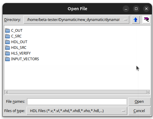
- Change the
Files of type:option toLog Files(*.wlf)and selectvsim.wlf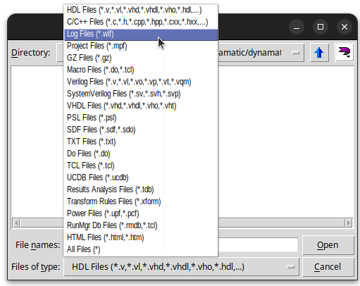
- Play around with the waveform in ModelSim
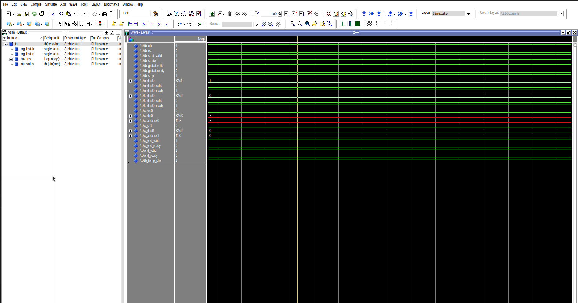
tip
The vsim.wlf file is also used by the interactive visualizer uses to animate the circuit using the Godot game engine.
- ModelSim information
- default settings
- library information to configure the simulator
- A script to compile and run the HDL simulation.
- A transcript of all commands run during the simulation.
- Testbench information
- optimization data
- temporary compilation data
- temporary message logs
- library metadata
- library hierarchy and elaboration logic
- dependency listing
report.txt
The report file gives information on the HDL simulation in ModelSim/Questa as well as some runtime and clock cycle information. If simulation fails, this file will also contain error logs to help the user understand the cause of failure.
Other Cosimulation Directories
The following directories contain information used to run the simuation:
1. C_SRC
Contains a copy of the C source file under test as well as any included header files. These will be used to compile and run the C program using a regular C compiler.
2. HDL_SRC
Contains a clone of the HDL directory created by the write-hdl command plus the addition of a testbench file that passes the inputs from the main function.
3. INPUT_VECTORS
Contains a list of .dat files for each input declared in the main function. These are passed to the C and HDL files during the co-simulation.
4. C_OUT
Contains the results of compiling and running the C program stored as .dat files for every output.
5. HDL_OUT
Contains the results of running the HDL simulation of the program in ModelSim/Questa stored as .dat files for every output.
Dynamatic compares the files in C_OUT and HDL_OUT to determine whether the HDL code generated does what the C program was intended to do.
Contributing
Dynamatic welcomes contributions from the open-source community and from students as part of academic projects. We generally follow the LLVM and MLIR community practices, and currently use GitHub issues and pull requests to handle bug reports/design proposals and code contributions, respectively. Here are some high-level guidelines (inspired by CIRCT’s guidelines):
- Please use
clang-formatin the LLVM style to format the code (see.clang-format). There are good plugins for common editors like VSCode (cpptool or clangd) that can be set up to format each file on save, or you can run them manually. This makes code easier to read and understand, and more uniform throughout the codebase. - Please pay attention to warnings from
clang-tidy(see.clang-tidy). Not all necessarily need to be acted upon, but in the majority of cases, they help in identifying code-smells. - Please follow the LLVM Coding Standards.
- Please practice incremental development, preferring to send a small series of incremental patches rather than large patches. There are other policies in the LLVM Developer Policy document that are worth skimming.
- Please create an issue if you run into a bug or problem with Dynamatic.
- Please create a PR to get a code review. For reviewers, it is good to look at the primary author of the code you are touching to make sure they are at least CC’d on the PR.
Relevant Documentation
You may find the following documentation useful when contributing to Dynamatic:
GitHub Issues & Pull requests
The project uses GitHub issues and pull requests (PRs) to handle contributions from the community. If you are unfamiliar with those, here are some guidelines on how to use them productively:
- Use meaningful titles and descriptions for issues and PRs you create. Titles should be short yet specific and descriptions should give a good sense of what you are bringing forward, be it a bug report or code contribution.
- If you intend to contribute a large chunk of code to the project, it may be a good idea to first open a GitHub issue to describe the high-level design of your contribution there and leave it up for discussion. This can only increase the likelihood of your work eventually being merged, as the community will have had a chance to discuss the design before you propose your implementation in a PR (e.g., if the contribution is deemed to large, the community may advise to split it up in several incremental patches). This is especially advisable to first-time contributors to open-source projects and/or compiler development beginners.
- Use “Squash and Merge” in PRs when they are approved - we don’t need the intra-change history in the repository history.
Experimental Work
One of Dynamatic’s priority is to keep the repository’s main branch stable at all times, with a high code quality throughout the project. At the same time, as an academic project we also receive regular code contributions from students with widely different backgrounds and field expertises. These contributions are often part of research-oriented academic projects, and are thus very “experimental” in nature. They will generally result in code that doesn’t quite match the standard of quality (less tested, reliable, interoperable) that we expect in the repository. Yet, we still want to keep track of these efforts on the main branch to make them visible to and usable by the community, and encourage future contributions to the more experimental parts of the codebase.
To achieve these dual and slightly conflicting goals, Dynamatic supports experimental contributions to the repository. These will still have to go through a PR but will be merged more easily (i.e., with slightly less regards to code quality) compared to non-experimental contributions. We offer this possibility as a way to push for the integration of research work inside the project, with the ultimate goal of having these contributions graduate to full non-experimental work. Obviously, we strongly encourage developers to make their submitted code contributions as clean and reliable as possible regardless of whether they are classified as experimental. It can only increase their chance of acceptance.
To clearly separate them from the rest, all experimental contributions should exist within the experimental directory which is located at the top level of the repository. The latter’s internal structure is identical to the one at the top level with an include folder for all headers, a lib folder for pass implementations, etc. All public code entities defined within experimental work should live under the dynamatic::experimental C++ namespace for clear separation with non-experimental publicly defined entities.
Software architecture
This section provides an overview of the software architecture of the project and is meant as an entry-point for users who would like to start digging into the codebase. It describes the project’s directory structure, our software dependencies (i.e., git submodules), and our testing infrastructure.
Directory structure
This section is intended to give an overview of the project’s directory structure and an idea of what each directory contains to help new users more easily look for and find specific parts of the implementation. Note that the superproject is structured very similarly to LLVM/MLIR, thus this overview is useful for navigating this repository as well. For exploring/editing the codebase, we strongly encourage the use of an IDE with a go to reference/implementation feature (e.g., VSCode) to easily navigate between header/source files. Below is a visual representation of a subset of the project’s directory structure, with basic information on what each directory contains.
├── bin # Symbolic links to commonly used binaries after build (untracked)
├── build # Files generated during build (untracked)
│   └── bin # Binaries generated by the superproject
│       └── include
│           └── dynamatic # Compiled TableGen headers (*.h.inc)
├── docs # Documentation and tutorials, where this file lies
├── experimental # Experimental passes and tools
├── include
│   ├── dynamatic # All header files (*.h)
├── integration-test # Integration tests
├── lib # Implementation of compiler passes (*.cpp)
│   ├── Conversion # Implementation of conversion passes (*.cpp)
│   └── Transforms # Implementation of transform passes (*.cpp)
├── polygeist # Polygeist repository (submodule)
│   └── llvm-project # LLVM/MLIR repository (submodule)
├── test # Unit tests
├── tools # Implementation of executables generated during build
│   └── dynamatic-opt # Dynamatic optimizer
├── tutorials # Dynamatic tutorials
├── visual-dataflow # Interactive dataflow visualizer (depends on Godot)
├── build.sh # Build script to build the entire project
└── CMakeLists.txt # Top level CMake file for building the superproject
Software Dependencies
See Dependencies.
Testing Infrastructure
See Testing
Dynamatic’s High Level Synthesis Flow
Flow script compile.sh
Diagram of the Overall Compilation Flow

Stage 1: Source -> Affine level
In this stage, we convert source code to affine level mlir dialect with polygist and generate the affine.mlir file.
Stage 2: Affine level -> SCF level
In this stage, we do the following two steps:
- Conduct pre-processing and memory analysis with
dynamatic_optand generateaffine_mem.mlir. - Convert the affine level mlir dialect to structured control flow(scf) level mlir dialect and generate the
scf.mlirfile.
Stage 3: SCF level -> CF level
In this stage, we convert the scf level mlir dialect to control flow(cf) level mlir dialect and generate the std.mlir file.
Stage 4: CF level transformations
In this stage we conduct the following two transformations in the cf level in order:
- Standard transformations and generate the
std_transformed.mlirfile. - Dynamatic specific transformations and generate the
std_dyn_transformed.mlirfile.
Stage 5: CF level -> Handshake level
In this stage we convert the cf level mlir dialect to handshake level mlir dialect and generate the handshake.mlir file.
Stage 6: Handshake level transformations
In this stage, we conduct handshake dialect related transformations and generate the handshake_transformed.mlir file.
Stage 7: Buffer Placement
In this stage, we conduct the buffer placement process, we have two `mutually excluseive`` options:
Smart buffer placement:- Profiling is performed at the CF level mlir dialect (specifically
std_dyn_transformed.mlir), and the results are exported to afreq.csvfile. - This
freq.csvfile is then used in the smart buffer placement process.
- Profiling is performed at the CF level mlir dialect (specifically
Simple buffer placement: (Dashed lines in the above diagram)- No need for profiling, we directly do buffer placement.
Results are stored in handshake_buffered.mlir file.
Stage 8: Export
In this stage, we conduct handshake canonicalization and produce the final export file (handshake_export.mlir).
Testing Infrastructure
Dynamatic features unit tests that evaluate the behavior of a small part of the implementation (typically, one compiler pass) against an expected output. All files within the test directory with the .mlir extension are automatically considered as unit test files. They can be ran/checked all at once by running ninja check-dynamatic from a terminal within the top level build directory. We use the FileCheck LLVM utility to compare the actual output of the implementation with the expected one.
Dynamatic also contains integration tests that assess the whole flow by going from C to VHDL. Each folder containing C source code inside the integration-test directory is a separate integration test.
Understanding FileCheck Unit Test Files
FileCheck is an LLVM utility that works by running a user-specified command (typically, a compiler pass through the dynamatic-opt tool) on each unit test present in a file and checking the output of the command (printed on stdout) against a pre-generated expected output expressed as a sequence of CHECK*: ... assertions. Test files are made up one or more unit tests that are each checked independently of the others. Each unit test is considered passed if and only if the output of the command matches the output contained in its associated CHECK assertions. The file is considered passed if and only if all unit tests contained within it passed.
We give an example test file (modeled after the real unit tests for the constant pushing pass located at test/Transforms/push-constants.mlir) and explain its content below.
// NOTE: Assertions have been autogenerated by utils/generate-test-checks.py
// RUN: dynamatic-opt --push-constants %s --split-input-file | FileCheck %s

// CHECK-LABEL:   func.func @simplePush(
// CHECK-SAME:                          %[[VAL_0:.*]]: i32) -> i32 {
// CHECK:           %[[VAL_1:.*]] = arith.constant 10 : i32
// CHECK:           %[[VAL_2:.*]] = arith.cmpi eq, %[[VAL_0]], %[[VAL_1]] : i32
// CHECK:           cf.cond_br %[[VAL_2]], ^bb1, ^bb2
// CHECK:         ^bb1:
// CHECK:           %[[VAL_3:.*]] = arith.constant 10 : i32
// CHECK:           return %[[VAL_3]] : i32
// CHECK:         ^bb2:
// CHECK:           %[[VAL_4:.*]] = arith.constant 10 : i32
// CHECK:           %[[VAL_5:.*]] = arith.subi %[[VAL_4]], %[[VAL_4]] : i32
// CHECK:           return %[[VAL_5]] : i32
// CHECK:         }
func.func @simplePush(%arg0: i32) -> i32 {
  %c10 = arith.constant 10 : i32
  %eq = arith.cmpi eq, %arg0, %c10 : i32
  cf.cond_br %eq, ^bb1, ^bb2
^bb1:
  return %c10 : i32
^bb2:
  %sub = arith.subi %c10, %c10 : i32
  return %sub : i32
}

// -----

// CHECK-LABEL:   func.func @pushAndDelete(
// CHECK-SAME:                             %[[VAL_0:.*]]: i1) -> i32 {
// CHECK:           cf.cond_br %[[VAL_0]], ^bb1, ^bb2
// CHECK:         ^bb1:
// CHECK:           %[[VAL_1:.*]] = arith.constant 0 : i32
// CHECK:           return %[[VAL_1]] : i32
// CHECK:         ^bb2:
// CHECK:           %[[VAL_2:.*]] = arith.constant 1 : i32
// CHECK:           return %[[VAL_2]] : i32
// CHECK:         }
func.func @pushAndDelete(%arg0: i1) -> i32 {
  %c0 = arith.constant 0 : i32
  %c1 = arith.constant 1 : i32
  cf.cond_br %arg0, ^bb1, ^bb2
^bb1:
  return %c0 : i32
^bb2:
  return %c1 : i32
}
- The
// RUN: ...statement at the top of the file contains the command to run for each unit test (here, for eachfunc.func). At test-time, the%sis replaced by the name of the test file. Here, the Dynamatic optimizer runs the--push-constantspass on each unit test and the transformed IR (printed to stdout bydynamatic-opt) is fed toFileCheckfor verification. // -----statements separate unit tests. They are read by the--split-input-filecompiler flag (provided by theRUNcommand) which wraps each unit test into an MLIRmodulebefore feeding each module to the specified pass(es) independently of one another.- Each
func.funcmodels a standard MLIR function, with its body enclosed between curly brackets, Here, eachfunc.funcrepresents a different unit test, since the constant pushing pass operates within the body of a single function at a time. - The
CHECK-LABEL,CHECK-SAME, andCHECKassertions represent the expected output for each unit test. They use some special syntax and conventions to verify that the output of each unit test is the one we expect while allowing some cosmetic differences between the expected and actual outputs that have no impact on behavior.FileCheck’s documentation explains how each assertion type is handled by the verifier. The section below explains how you can generate these assertions automatically for your own unit tests.
Creating Your Own Unit Tests With FileCheck
Unit tests are a very useful way to check the behavior of a specific part of the codebase, for example, a transformation pass. They allow us to verify that the code produces the right result in small, specific, and controlled scenarios that ideally fully cover the design under test (DUT). Furthermore, unit tests are very easy to write and maintain with the FileCheck LLVM utility, making them a requirement when contributing non-trivial code to the project. We go into how to write you own unit tests and automatically generate FileCheck annotations (i.e., CHECK assertions) for them below.
Writing Good Unit Tests
As their name suggests, unit tests are meant to test one unit of functionality. Typically, this means that the DUT must be as minimal as possible while remaining practical to analyze (e.g., there is no need to test each individual function). In most cases this translates to testing a single compiler pass in isolation, for example, the constant pushing (--push-constants) pass. Each unit test should aim, as much as possible, to evaluate a single behavior of the DUT. Consequently, it is good practice to make unit tests as small as possible for testing for a desired functionality. Doing so makes it easier for future readers to understand (1) what behavior the unit test checks for and (2) where to look in the code if a test starts failing.
TODO | Formalize List of Unit Tests to Have for a Pass, an Operation, Etc.
Generating FileCheck Assertions
Once you have written your own unit tests, all that remains to do is generate FileCheck annotations that will allow the latter to verify that the output of the DUT matches the expected one. Let’s take the example test file given above without FileCheck annotations as an example and go through the process of generating assertions for its two unit tests. We start from a test file containing only the input code that will go through the constant pushing pass as well as a // ----- marker to later instruct the Dynamatic optimizer to split the file into separarte MLIR modules in this location.
func.func @simplePush(%arg0: i32) -> i32 {
  %c10 = arith.constant 10 : i32
  %eq = arith.cmpi eq, %arg0, %c10 : i32
  cf.cond_br %eq, ^bb1, ^bb2
^bb1:
  return %c10 : i32
^bb2:
  %sub = arith.subi %c10, %c10 : i32
  return %sub : i32
}

// -----

func.func @pushAndDelete(%arg0: i1) -> i32 {
  %c0 = arith.constant 0 : i32
  %c1 = arith.constant 1 : i32
  cf.cond_br %arg0, ^bb1, ^bb2
^bb1:
  return %c0 : i32
^bb2:
  return %c1 : i32
}
Test files need to be located in the the test folder of the repository. Constant pushing is a transformation pass, so we store it as test/Transforms/example.mlir.
From the top level of the repository, assuming you have already built the project, you can now run:
./build/bin/dynamatic-opt test/Transforms/example.mlir --push-constants --split-input-file | circt/llvm/mlir/utils/generate-test-checks.py --source=test/Transforms/example.mlir --source_delim_regex="func.func"
Let’s break this command down, token by token:
./build/bin/dynamatic-optruns any (sequence of) compiler pass(es) defined by Dynamatic on a source MLIR file passed as argument and prints the transformed IR on standard output.test/Transforms/example.mlirindicates the file containing the IR you want to transform using the constant pushing pass.--push-constantsinstructs the optimizer to run the constant pushing pass.--split-input-fileinstructs the compiler to wrap each piece of code separated by a line containing only// -----into an MLIR module.|pipes the standard output of the command on its left (i.e., the input code transformed by the constant pushing pass) to the standard input of the command on its right (i.e., the code to transform intoFileCheckassertions).circt/llvm/mlir/utils/generate-test-checks.pytransforms the IR it is given on standard input into a sequence ofCHECKassertions and prints them to standard output.--source=test/Transforms/example.mlirindicates the source unit test file for which assertions are being generated, and is used to print the source code of each unit test below its corresponding assertions after transformation on standard output--source_delim_regex="func.func"indicates a regex on which to split the source code. Each split of the source code will be grouped with its correspondingCHECKassertions in the output, and splits will be displayed one after the other. Here, since each standard MLIR function represents a unit test, we split on afunc.func.
After running the command, the following should be printed to standard output.
// NOTE: Assertions have been autogenerated by utils/generate-test-checks.py

// The script is designed to make adding checks to
// a test case fast, it is *not* designed to be authoritative
// about what constitutes a good test! The CHECK should be
// minimized and named to reflect the test intent.

// NOTE: Assertions have been autogenerated by utils/generate-test-checks.py
// RUN: dynamatic-opt --push-constants %s --split-input-file | FileCheck %s

// CHECK-LABEL:   func.func @simplePush(
// CHECK-SAME:                          %[[VAL_0:.*]]: i32) -> i32 {
// CHECK:           %[[VAL_1:.*]] = arith.constant 10 : i32
// CHECK:           %[[VAL_2:.*]] = arith.cmpi eq, %[[VAL_0]], %[[VAL_1]] : i32
// CHECK:           cf.cond_br %[[VAL_2]], ^bb1, ^bb2
// CHECK:         ^bb1:
// CHECK:           %[[VAL_3:.*]] = arith.constant 10 : i32
// CHECK:           return %[[VAL_3]] : i32
// CHECK:         ^bb2:
// CHECK:           %[[VAL_4:.*]] = arith.constant 10 : i32
// CHECK:           %[[VAL_5:.*]] = arith.subi %[[VAL_4]], %[[VAL_4]] : i32
// CHECK:           return %[[VAL_5]] : i32
// CHECK:         }
func.func @simplePush(%arg0: i32) -> i32 {
  %c10 = arith.constant 10 : i32
  %eq = arith.cmpi eq, %arg0, %c10 : i32
  cf.cond_br %eq, ^bb1, ^bb2
^bb1:
  return %c10 : i32
^bb2:
  %sub = arith.subi %c10, %c10 : i32
  return %sub : i32
}

// -----

// CHECK-LABEL:   func.func @pushAndDelete(
// CHECK-SAME:                             %[[VAL_0:.*]]: i1) -> i32 {
// CHECK:           cf.cond_br %[[VAL_0]], ^bb1, ^bb2
// CHECK:         ^bb1:
// CHECK:           %[[VAL_1:.*]] = arith.constant 0 : i32
// CHECK:           return %[[VAL_1]] : i32
// CHECK:         ^bb2:
// CHECK:           %[[VAL_2:.*]] = arith.constant 1 : i32
// CHECK:           return %[[VAL_2]] : i32
// CHECK:         }
func.func @pushAndDelete(%arg0: i1) -> i32 {
  %c0 = arith.constant 0 : i32
  %c1 = arith.constant 1 : i32
  cf.cond_br %arg0, ^bb1, ^bb2
^bb1:
  return %c0 : i32
^bb2:
  return %c1 : i32
}
It is now fundamental that you manually check the generated assertions and verify that they match the output that you expect from the DUT. Indeed, at this point no verification of any kind has happened. The previous command simply ran the constant pushing pass on each unit test and turned the resulting IR into CHECK assertions, which will from this moment forward be considered the expected output of the pass on the unit tests. At this time you are thus the verifier who needs to make sure these assertions showcase the correct and intended behavior of the DUT.
Once you are confident that the DUT’s output is correct on the unit tests, you can overwrite the content of test/Transforms/example.mlir with the command output (skipping the NOTE on the first line and the following commented out paragraph). If you now go to the build directory at the top level of the repository and run ninja check-dynamatic, you unit tests should be executed, checked, and (at this point) pass.
Congratulations! You have now
- created good unit tests to make sure a part of the codebase works as intended and,
- set up an easy way for you and future developers of Dynamatic to make sure it keeps working as we move forward!
A Known Assertion Generation Bug
The assertion generation script (circt/llvm/mlir/utils/generate-test-checks.py) sometimes generates CHECK assertions that FileCheck is then unable to verify, even when running ninja check-dynamatic immediately after creating assertions (which, logically, should always verify). The issue arises in some cases with functions of more than two arguments and has a simple formatting fix. For example, consider the following unit test with its associated automatically generated assertions (body assertions skipped for brevity).
// CHECK-LABEL:   handshake.func @duplicateLiveOut(
// CHECK-SAME:                                     %[[VAL_0:.*]]: i1,
// CHECK-SAME:                                     %[[VAL_1:.*]]: i32,
// CHECK-SAME:                                     %[[VAL_2:.*]]: i32,
// CHECK-SAME:                                     %[[VAL_3:.*]]: none, ...) -> none {
// [...]
// CHECK:         }
func.func @duplicateLiveOut(%arg0: i1, %arg1: i32, %arg2: i32) {
  cf.cond_br %arg0, ^bb1(%arg1, %arg2, %arg1: i32, i32, i32), ^bb1(%arg2, %arg2, %arg2: i32, i32, i32)
  ^bb1(%0: i32, %1: i32, %2: i32):
    return
}
The unit test above reports a matching error near %[[VAL_2:.*]]: i32 and fails to verify regardless of the function body assertions’ correctness. Merging the second and third function argument on a single line as follows solves the issue.
// CHECK-LABEL:   handshake.func @duplicateLiveOut(
// CHECK-SAME:                                     %[[VAL_0:.*]]: i1,
// CHECK-SAME:                                     %[[VAL_1:.*]]: i32, %[[VAL_2:.*]]: i32,
// CHECK-SAME:                                     %[[VAL_3:.*]]: none, ...) -> none {
// [...]
// CHECK:         }
func.func @duplicateLiveOut(%arg0: i1, %arg1: i32, %arg2: i32) {
  cf.cond_br %arg0, ^bb1(%arg1, %arg2, %arg1: i32, i32, i32), ^bb1(%arg2, %arg2, %arg2: i32, i32, i32)
  ^bb1(%0: i32, %1: i32, %2: i32):
    return
}
Creating Dynamatic Compiler Passes
This tutorial will walk you through the creation of a simple transformation pass for Dynamatic that simplifies merge-like operations in Handshake-level IR. We’ll look at the process of declaring a pass in TableGen format, creating a header file for the pass that includes the auto-generated pass declaration code, and implementing the transformation as part of an mlir::OperationPass. Then, we’ll look at how to use a greedy pattern rewriter to make our pass easier to write and able to optimize the IR in more situations.
This tutorial assumes basic knowledge of C++, MLIR, and of the theory behind dataflow circuits. For a basic introduction to MLIR and its related jargon, see the MLIR primer. The full (runnable!) source code for this tutorial is located in tutorials/include/tutorials/CreatingPasses (headers) as well as in tutorials/lib/CreatingPasses (sources), and is built alongside the rest of the project by default.
This tutorial is divided in the following chapters:
- Chapter #1 | Description of what we want to achieve with the transformation pass: simlifying merge-like operations in the IR.
- Chapter #2 | Writing an initial version of the pass that transforms the IR in (almost!) the intended way.
- Chapter #3 | Improving the pass design and fixing our previous issue using a
GreedyPatternRewriterDriver.
Simplifying Merge-Like Operations
The first chapter of this tutorial describes what transformation we are going to implement in our dataflow circuits, which, in Dynamatic, are modeled using the Handshake MLIR dialect.
Merge-like Dataflow Components
There are three dataflow components which fall under the category of “merge-like” components.
- The merge is a nondeterministic component which propagates a token received on any of its $N$ inputs to its single output.
- The control merge (or cmerge) behaves like the merge with the addition of a second output that indicates which of the inputs was selected (via the input’s index, from $0$ to $N-1$).
- The mux is a deterministic version of the merge that propogates to its single output the input token selected by a control input (via the input’s index, from $0$ to $N-1$).
Merge-like components are generally found at the beginning of basic blocks and serve the purpose of merging the data and control flow coming from diverging paths in the input code (e.g., after an if/else statement).
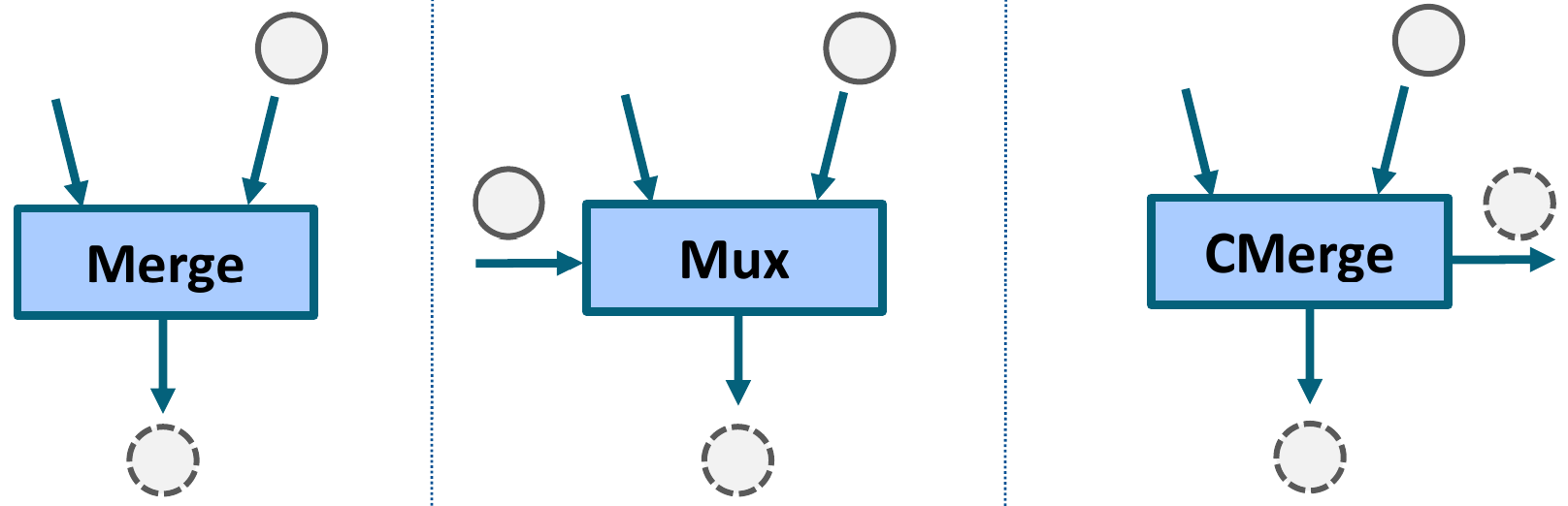 Image from Lana Josipović, Andrea Guerrieri, and Paolo Ienne. Dynamatic: From C/C++ to Dynamically-Scheduled Circuits. Invited tutorial. In Proceedings of the 28th ACM/SIGDA International Symposium on Field Programmable Gate Arrays, Seaside, Calif., February 2020
Merge-like operations
These three dataflow components map one-to-one to identically-named MLIR operations that are part of the Handshake dialect.
- The merge operation (
circt::handshake::MergeOp, declared here) which accepts a strictly positive number of operands (all with the same type) and returns a single result of the same type. Below is the syntax for a merge with twoi32operands.%input0 = [...] : i32 %input1 = [...] : i32 %mergeResult = merge %input0, %input1 : i32 - The mux operation (
circt::handshake::MuxOp, declared here) which accepts an integer-like select operand (acting as the selector for which input token to propogate to the output) and a strictly positive number of data operands (all with the same type). It returns a single result of the same type as the data operands. Below is the syntax for a mux with twoi32operands.%sel = [...] : index %input0 = [...] : i32 %input1 = [...] : i32 %muxResult = mux %sel [%input0, %input1] : index, i32 - The control merge operation (
circt::handshake::ControlMergeOp, declared here) which accepts a strictly positive number of operands (all with the same type) and returns a data result of the same type, as well as an integer-like index result. Below is the syntax for a control merge with twoi32operands.%input0 = [...] : i32 %input1 = [...] : i32 %cmergeResult, %cmergeIndex = control_merge %input0, %input1 : i32, index
Simplifying Merge-like Operations
Generally speaking, we always strive to make dataflow circuits faster (in runtime) and smaller (in area). We are thus going to implement a circuit transformation pass that will remove some useless dataflow components (that would otherwise increase circuit delay and area) and downgrade others to simpler equivalent components (that take up less area). The particular transformation we will implement in this tutorial is going to operate on merge-like operations in the Handshake-level IR. It is made up of two separate optimizations that we describe below.
Erasing Single-Input Merges
Merge operations non-deterministically forward one of their valid input tokens to their single output. It is easy to see that a merge with a single input is behaviorally equivalent to a wire, since a valid input token will always be forwarded to the output. Such merges can safely be deleted without affecting circuit functionality.
Consider the following trivial example of a Handshake function that simply returns its %start input.
handshake.func @eraseSingleInputMerge(%start: none) -> none {
  %mergeStart = merge %start : none
  %returnVal = return %mergeStart : none
  end %returnVal : none
}
The first operation inside the function is a merge with a single input. As discussed above, it can be erased to simplify the circuit. Our pass should transform the above IR into the following.
handshake.func @eraseSingleInputMerge(%start: none) -> none {
  %returnVal = return %start : none
  end %returnVal : none
}
Notice that the circuit had to be “re-wired” so that return now takes as input the single operand to the now deleted merge instead of its result.
You may wonder how our dataflow circuits could ever end up with such useless components within them, and, consequently, why we would ever need to implement such an optimization for something that should never have been there in the first place. It is in fact not an indication of bad design that operations which can be optimized away are temporarily present in the IR. These may be remnants of prior transformation passes that operated on a different aspect of the IR and whose behavior resulted in a merge losing some of its inputs as a side-effect. In this particular case, it is our lowering pass from std-level to Handshake-level that adds single input merges to the IR in specific situations for the sake of having all basic blocks live-ins go through merge-like operations before “entering” a block. Generally speaking, it should be the job of a compiler’s canonicalization infrastructure to optimize the IR in such a way, but for the sake of this tutorial we will implement the merge erasure logic as part of our transformation pass.
Downgrading Index-less Control Merges
In addition to behaving like a merge, control merges also output the index of the input token that was non-deterministically chosen. If this output (the second result of the control_merge MLIR operation) is unused in the circuit, then a control merge is semantically equivalent to a merge, and can safely be downgraded to one, gaining some area in the process. Going forward, we will refer to such control merges as being “index-less”.
Consider the following trivial example of a Handshake function that non-deterministicaly picks and returns one of its two first inputs.
handshake.func @downgradeIndexLessControlMerge(%arg0: i32, %arg1: i32, %start: none) -> i32 {
  %cmergeRes, %cmergeIdx = control_merge %arg0, %arg1 : i32, index
  %returnVal = return %cmergeRes : i32
  end %returnVal : i32
}
The control_merge’s index result (%cmergeIdx) is unused in the IR. As discussed above, the operation can safely be downgraded to a merge. Our pass should transform the above IR into the following.
handshake.func @downgradeIndexLessControlMerge(%arg0: i32, %arg1: i32, %start: none) -> i32 {
  %mergeRes = merge %arg0, %arg1 : i32, index
  %returnVal = return %mergeRes : i32
  end %returnVal : i32
}
Conclusion
In this chapter, we described the circuit optimizations we would like to achieve in our MLIR transformation pass. In summary, we want to (1) erase merge operation with a single operand and (2) downgrade index-less control_merge operations to simpler merge operations. In the next chapter we will go through the process of writing, building, and running this pass in Dynamatic.
Writing a Simple MLIR Pass
The second chapter of this tutorial describes the implementation of a simple transformation pass in Dynamatic. This pass operates on Handshake-level IR and simplifies merge-like operations to make our dataflow circuits faster and smaller. We will
- declare the pass in TableGen, which will automatically generate a lot of boilerplate C++ code at compile-time,
- declare a header for the pass that includes some auto-generated code and declares the pass constructor,
- implement the pass constructor and its skeleton using some of the auto-generated code,
- configure the project to be able to run our pass with
dynamatic-opt, the Dynamatic optimizer, - and, finally, implement our circuit transformation.
You can write the entire pass yourself from the code snippets provided in this tutorial. The write-up assumes that no files related to the pass exist initially and walks you through the creation and implementation of those files. However, the full source code for this tutorial is provided in tutorials/CreatingPasses/include/tutorials/CreatingPasses and tutorials/CreatingPasses/lib/CreatingPasses for reference. To avoid name clashes while easily matching between the reference code and the code you may choose to write while reading this tutorial, all relevant names will be prefixed by My in the snippets present in this file compared to names used in the reference code. For example, the pass will be named MySimplifyMergeLike in this tutorial whereas it is named SimplifyMergeLike in the reference code.
The project is configured to build all tutorials along the rest of the project. By the end of this chapter, you will be able to run your own pass using Dynamatic’s optimizer!
Declaring our Pass in TableGen
The first step in the creation of our pass is to declare it inside a TableGen file (with .td extension). TableGen is an LLVM tool whose “purpose is to help a human develop and maintain records of domain-specific information”. For our purposes, we can see TableGen as a preprocessor that inputs text files (with the .td extension by convention) containing information on user-defined MLIR entities (e.g., compiler passes, dialect operations, etc.) and outputs automatically-generated boilerplate C++ code that “implements” these entities. TableGen’s input format is mostly declarative; it declares the existence of entities and characterizes their properties, but largely does not directly describe how these entities behave. The behavior of TableGen-defined entities must be written in C++, which we will do in the following sections. For this tutorial, we will have TableGen automatically generate the C++ code corresponding to our pass declaration. TableGen will also automatically generate a registration function that will enable the Dynamatic optimizer to register and run our pass.
Inside tutorials/CreatingPasses/include/tutorials/, which already exists, start by creating a directory named MyCreatingPasses which will contain all declarations for this tutorial. It’s conventional to put the declaration of all transformation passes in a sub-directory called Transforms, so create one such directory within MyCreatingPasses. Finally, create a TableGen file named Passes.td inside that last directory. At this point, the filesystem should look like the following.
├── tutorials
│   ├── CreatingPasses
│     ├── include
│         ├── tutorials
│             ├── CreatingPasses # Reference code for this tutorial
│             ├── MyCreatingPasses # The first directory you just created
│                 └── Transforms # The second directory you just created
│                     └── Passes.td # The file you just created
│             ├── CMakeLists.txt
│             └── InitAllPasses.h
│     ├── lib
│     └── test
├── build.sh
├── README.md
└── ... # Other files/folders at the top level
We will declare our pass inside Passes.td. Copy and paste the following snippet into the file.
//===- Passes.td - Transformation passes definition --------*- tablegen -*-===//
//
// This file contains the definition for all transformation passes in this
// tutorial.
//
//===----------------------------------------------------------------------===//

#ifndef TUTORIALS_MYCREATINGPASSES_TRANSFORMS_PASSES_TD
#define TUTORIALS_MYCREATINGPASSES_TRANSFORMS_PASSES_TD

include "mlir/Pass/PassBase.td"

def MySimplifyMergeLike : Pass< "tutorial-handshake-my-simplify-merge-like",
                                "mlir::ModuleOp"> {
  let summary = "Simplifies merge-like operations in Handshake functions.";
  let description = [{
    The pass performs two simple transformation steps sequentially in each
    Handshake function present in the input MLIR module. First, it bypasses and
    removes all merge operations (circt::handshake::MergeOp) with a single
    operand from the IR, since they serve no purpose. Second, it downgrades all
    control merge operations (circt::handshake::ControlMergeOp) whose index
    result is unused into simpler merges with the same operands.
  }];
  let constructor = "dynamatic::tutorials::createMySimplifyMergeLikePass()";
}

#endif // TUTORIALS_MYCREATINGPASSES_TRANSFORMS_PASSES_TD
Let’s go over the file’s content. You may see that it shares syntactic similarity with C/C++. Like all C++ files in the repository, the file starts with a header comment containing some meta information as well as a description of the file’s content. Like a header, it contains an include guard (#ifndef <guard>/#define <guard>/#endif) and includes another TableGen file (include "mlir/Pass/PassBase.td", note the lack of a # before the include keyword). The heart of the file is the declaration of the MySimplifyMergeLikePass which inherits from a Pass. The Pass object is given 2 generic arguments between <>.
- First is the flag name that will reference the pass in the Dynamatic optimizer
tutorial-handshake-my-simplify-merge-like. Note that the actual flag name will be prefixed by a double-dash, so that it’s possible to run the pass on some input Handshake-level IR with$ ./bin/dynamatic-opt handshake-input.mlir --tutorial-handshake-my-simplify-merge-like - Second is the MLIR operation that this pass matches on (i.e., the operation type the pass driver will look for in the input to run the pass on). In the vast majority of cases, we want passes to match an
mlir::ModuleOp, which is always the top level operation under which everything is nested in our MLIR inputs.
The pass declaration contains some pass members which one must always define (there exists other members, but they are out of the scope of this tutorial). These are:
- The
summary, containing a one-line short description of what the pass does. - The
description, containing a more detailed description of what the pass does. - The
constructor, indicating the full qualified name of a function that returns a unique instance of the pass. We will declare and define this function in the next sections of this chapter. Notice that we create the function under thedynamatic::tutorialsnamespace. Every public member of Dynamatic should live in thedynamaticnamespace. As to not pollute the repository’s main namespace, everything related to the tutorials is further placed inside the nestedtutorialsnamespace.
We now need to write some CMake configuration code to instruct the build system to automatically generate C++ code that corresponds to this TableGen file, and then compile this generated C++ along the rest of the project. First, create a file named CMakeLists.txt next to Passes.td with the following content.
set(LLVM_TARGET_DEFINITIONS Passes.td)
mlir_tablegen(Passes.h.inc -gen-pass-decls)
add_public_tablegen_target(DynamaticTutorialsMyCreatingPassesIncGen)
add_dependencies(dynamatic-headers DynamaticTutorialsMyCreatingPassesIncGen)
You do not need to understand precisely how this works. It suffices to know that it instructs the build system to create a target named DynamaticTutorialsMyCreatingPassesIncGen that libraries can depend on to get definitions related to Passes.td’s content. To get this file included in the build when running $ cmake ..., we must include its parent directory from CMake files higher in the hierarchy. Modify the existing CMakeLists.txt in tutorials/CreatingPasses to add the subdirectory we just created.
include_directories(include)
include_directories(${DYNAMATIC_BINARY_DIR}/tutorials/CreatingPasses/include)

add_subdirectory(include/tutorials/CreatingPasses)
add_subdirectory(include/tutorials/MyCreatingPasses)   # you need to add this.
add_subdirectory(lib)
Similarly, create another CMakeLists.txt in tutorials/CreatingPasses/include/tutorial/MyCreatingPasses to include add nested subdirectory we created.
add_subdirectory(Transforms)
Everything we just did will eventually automatically generate a C++ header corresponding to Passes.td. It will be created inside the build directory (build/tutorials/CreatingPasses/include/tutorials/MyCreatingPasses/Transforms/Passes.h.inc) and will contain a lot of boilerplate code that you will rarely ever have to look at. Re-building the project right now would not generate the header because the build system would be able to identify that no part of the framework depends on it yet. We will see how to include parts of this header file inside our own C++ code using preprocessor flags in the next section, after which building the project will result in the header being genereted.
Declaring our Pass in C++
Now that we got TableGen to generate the boilerplate code for this pass, we can finally start writing some C++ of our own. Create a header file called MySimplifyMergeLike.h next to Passes.td. We will include the auto-generated pass declaration and declare our pass constructor there using the following code.
//===- MySimplifyMergeLike.h - Simplifies merge-like ops --------*- C++ -*-===//
//
// This file declares the --tutorial-handshake-my-simplify-merge-like pass.
//
//===----------------------------------------------------------------------===//

#ifndef TUTORIALS_MYCREATINGPASSES_TRANSFORMS_MYSIMPLIFYMERGELIKE_H
#define TUTORIALS_MYCREATINGPASSES_TRANSFORMS_MYSIMPLIFYMERGELIKE_H

#include "dynamatic/Support/LLVM.h"
#include "mlir/Pass/Pass.h"

namespace dynamatic {
namespace tutorials {

#define GEN_PASS_DECL_MYSIMPLIFYMERGELIKE
#define GEN_PASS_DEF_MYSIMPLIFYMERGELIKE
#include "tutorials/MyCreatingPasses/Transforms/Passes.h.inc"

std::unique_ptr<mlir::OperationPass<mlir::ModuleOp>>
createMySimplifyMergeLikePass();

} // namespace tutorials
} // namespace dynamatic

#endif // TUTORIALS_MYCREATINGPASSES_TRANSFORMS_MYSIMPLIFYMERGELIKE_H
Beyond the standard C++ header structure, this file does two important things.
- It includes the auto-generated pass declaration code inside the
dynamatic::tutorialsnamespace.
Notice the preprocessor flag defined just before including the file. It serves the purpose of isolating a single part of the auto-generated header to include in our own header, here the declaration of our pass. The preprocessor’s flag name is also auto-generated using the#define GEN_PASS_DECL_MYSIMPLIFYMERGELIKE #define GEN_PASS_DEF_MYSIMPLIFYMERGELIKE #include "tutorials/MyCreatingPasses/Transforms/Passes.h.inc"GEN_PASS_[DEF|DECL]_<my_pass_name_in_all_caps>template. If we were to define more passes insidePasses.td, all of them would get a declaration inside"tutorials/MyCreatingPasses/Transforms/Passes.h.inc". This preprocessor flag allows us to pick the single declaration we care about in the context. - It declares our pass’s constructor function, whose name we declared inside
Passes.td. Do not pay much attention to the constructor’s complicated-looking return type at this point, it is in fact trivial to implement this function.
Implementing the Skeleton of our Pass
We are now ready to start implementing our circuit transformation! We first write down some boilerplate skeleton code and configure CMake to build our implementation.
Inside tutorials/CreatingPasses/lib/, which already exists, start by creating two nested directories named MyCreatingPasses/Transforms (notice that the file structure is the same as in the tutorials/CreatingPasses/include/tutorials/ directory). Now, create a C++ source file named MySimplifyMergeLike.cpp inside the nested directory you just created to contain the implementation of our pass. Copy and paste the following code inside the source file.
//===- MySimplifyMergeLike.cpp - Simplifies merge-like ops ------*- C++ -*-===//
//
// Implements the --tutorial-handshake-my-simplify-merge-like pass, which uses a
// simple OpBuilder object to modify the IR within each handshake function.
//
//===----------------------------------------------------------------------===//

#include "tutorials/MyCreatingPasses/Transforms/MySimplifyMergeLike.h"
#include "dynamatic/Dialect/Handshake/HandshakeOps.h"
#include "mlir/IR/BuiltinOps.h"
#include "mlir/IR/MLIRContext.h"

using namespace mlir;
using namespace dynamatic;

namespace {

/// Simple pass driver for our merge-like simplification transformation. At this
/// point it only prints a message to stdout.
struct MySimplifyMergeLikePass
    : public dynamatic::tutorials::impl::MySimplifyMergeLikeBase<
          MySimplifyMergeLikePass> {

  void runOnOperation() override {
    // Get the MLIR context for the current operation being transformed
    MLIRContext *ctx = &getContext();
    // Get the operation being transformed (the top level module)
    ModuleOp mod = getOperation();
    // Print a message on stdout to prove that the pass is running
    llvm::outs() << "My pass is running!\n";
  };
};
} // namespace

namespace dynamatic {
namespace tutorials {

/// Returns a unique pointer to an operation pass that matches MLIR modules. In
/// our case, this is simply an instance of our unparameterized
/// MySimplifyMergeLikePass driver.
std::unique_ptr<mlir::OperationPass<mlir::ModuleOp>>
createMySimplifyMergeLikePass() {
  return std::make_unique<MySimplifyMergeLikePass>();
}
} // namespace tutorials
} // namespace dynamatic
Let’s take a close look at the content of this source file, which for now only contains the skeleton of our pass. At the very bottom, we see the definition of our pass constructor that we declared in MySimplifyMergeLike.h. It simply returns a unique pointer to an instance of a MySimplifyMergeLikePass, which is a struct defined above inside an anonymous namespace. You can view this struct as the driver for our pass, and an instance of MySimplifyMergeLikePass as a particular instance of our pass. Let’s break down the struct declaration and definition.
- The struct declaration is quite verbose, but it will always have the same structure for any pass you implement.
The namestruct MySimplifyMergeLikePass : public dynamatic::tutorials::impl::MySimplifyMergeLikeBase< MySimplifyMergeLikePass> {...}MySimplifyMergeLikePassdoes not have any particular importance, but it is conventional to use the pass name as declared in the TableGen file (that we created in this section) suffixed byPass. The struct inherits fromMySimplifyMergeLikeBase, which is defined inside thedynamatic::tutorials::implnamespace. You may not remember defining this class anywhere. This is because it is the pass declaration that was auto-generated from TableGen inside"tutorials/MyCreatingPasses/Transforms/Passes.h.inc"and included fromMySimplifyMergeLike.h, which the source file then includes. The nameMySimplifyMergeLikeBaseis auto-generated from the pass name declared in the TableGen file, to whichBaseis suffixed (it is the base class we inherit from). Finally, the base class is templated using… the derived struct’s itself? This may seem counter-intuitive, and you may wonder how this could even compile, but it is in fact a well-known C++ idiom called the curiously recurring template pattern that is used throughout MLIR. - The struct overrides a single method named
runOnOperation. It is the method that will be called on eachmlir::ModuleOpfound in the input IR, since we declared our pass (inPasses.td) to match this operation type. Right now, the method just retrieves the current MLIR context and operation it was matched on, and prints a message to standard output. In the next section, we will implement our circuit transformation within this method.
Running Our Pass
Configuring CMake
We now configure CMake to build this pass along the rest of the project. We have to create a CMakeLists.txt file in each directory we created and modify the one at tutorials/CreatingPasses/lib. Starting with the latter, just add a line to include the new directory structure in the build.
add_subdirectory(CreatingPasses)
add_subdirectory(MyCreatingPasses)
Similarly, inside tutorials/CreatingPasses/lib/MyCreatingPasses/CMakeLists.txt, just write the following to include the Transforms subdirectory, where our pass implemenation lies.
add_subdirectory(Transforms)
Finally, add the following snippet to tutorials/CreatingPasses/lib/MyCreatingPasses/Transforms/CMakeLists.txt.
add_dynamatic_library(DynamaticTutorialsMyCreatingPasses
  MySimplifyMergeLike.cpp

  DEPENDS
  DynamaticTutorialsMyCreatingPassesIncGen

  LINK_LIBS PUBLIC
  MLIRIR
  MLIRSupport
  MLIRTransformUtils
)
This CMake file creates a new Dynamatic library called DynamaticTutorialsMyCreatingPasses, which includes our pass implementation (MySimplifyMergeLike.cpp) and depends on DynamaticTutorialsMyCreatingPassesIncGen (the TableGen target we created earlier in tutorials/CreatingPasses/include/tutorials/CreatingPasses/Transforms/CMakeLists.txt) as well as a couple of standard MLIR targets which are built as part of our software dependencies.
The last CMake step is to add your new dynamatic library to the optimizer by modifying tools/dynamatic-opt/CMakeLists.txt. This will allow the optimizer to include your pass implementation in its binary. Add your library to the list of existing libraries that the dynamatic-opt tool gets linked to as follows.
target_link_libraries(dynamatic-opt
  PRIVATE
  DynamaticTransforms
  DynamaticTutorialsCreatingPasses
  DynamaticTutorialsMyCreatingPasses # your library!

  <... other libraries>
)
Registering Our Pass
To be able to run a pass, the optimizer needs to register it at compile-time. The tool is already configured to register all tutorial passes by calling the dynamatic::tutorials::registerAllPasses() function located in tutorials/CreatingPasses/include/tutorials/InitAllPasses.h, so we just have to add our own pass to this function. To do that, first create a file named Passes.h inside tutorials/CreatingPasses/include/tutorials/MyCreatingPasses/Transforms/, and paste the following into it.
//===- Passes.h - Transformation passes registration ------------*- C++ -*-===//
//
// This file contains declarations to register transformation passes.
//
//===----------------------------------------------------------------------===//

#ifndef TUTORIALS_MYCREATINGAPASSES_TRANSFORMS_PASSES_H
#define TUTORIALS_MYCREATINGAPASSES_TRANSFORMS_PASSES_H

#include "dynamatic/Support/LLVM.h"
#include "mlir/Pass/Pass.h"
#include "tutorials/MyCreatingPasses/Transforms/MySimplifyMergeLike.h"

namespace dynamatic {
namespace tutorials {

namespace MyCreatingPasses {

/// Generate the code for registering passes.
#define GEN_PASS_REGISTRATION
#include "tutorials/MyCreatingPasses/Transforms/Passes.h.inc"

} // namespace MyCreatingPasses
} // namespace tutorials
} // namespace dynamatic

#endif // TUTORIALS_MYCREATINGAPASSES_TRANSFORMS_PASSES_H
Similarly to MySimplifyMergeLike.h, this file includes some auto-generated code from "tutorials/MyCreatingPasses/Transforms/Passes.h.inc". This time, however, the GEN_PASS_REGISTRATION pre-processor flag indicates that the pass registration functions should be included instead of the pass declarations.
Next, open tutorials/CreatingPasses/include/tutorials/InitAllPasses.h and add the file you just created to the list of include statements.
#include "tutorials/MyCreatingPasses/Transforms/Passes.h"
Finally, inside the file tutorials/CreatingPasses/include/tutorials/CreatingPasses/InitAllPasses.h in the function registerAllPasses, add the following line to register your pass using the auto-generated registerPasses method.
dynamatic::tutorials::MyCreatingPasses::registerPasses();
We created a lot of directories and files in the last two sections, so let’s recap what our file system should look like at this point.
├── tutorials
│   ├── CreatingPasses
│     ├── include
│         └── tutorials
│             ├── CreatingPasses # Reference code for this tutorial
│             ├── MyCreatingPasses
│                 ├── CMakeLists.txt
│                 └── Transforms
│                     ├── CMakeLists.txt
│                     ├── MySimplifyMergeLike.h
│                     ├── Passes.td
│                     └── Passes.h # The file you just created
│             ├── CMakeLists.txt
│             └── InitAllPasses.h # Modified just now to register your pass
│     ├── lib
│         ├── CMakeLists.txt # Modified to add_subdirectory(MyCreatingPasses)
│         ├── CreatingPasses # Reference code for this tutorial
│         └── MyCreatingPasses # All created by you
│             ├── CMakeLists.txt # add_subdirectory(Transforms)
│             └── Transforms
│                     ├── CMakeLists.txt # add_dynamatic_library(...)
│                     └── MySimplifyMergeLike.cpp # Pass skeleton
│     └── test
├── build.sh
├── README.md
└── ... # Other files/folders at the top level
You should now be able to compile your skeleton pass implementation using the repository’s build script (./build.sh, from the top-level directory). Once successfully compiled, and to verify that everything works as intended, try to run your pass on the test file located at tutorials/test/creating-passes.mlir using the following command (run from the repository’s top level).
$ ./bin/dynamatic-opt tutorials/CreatingPasses/test/creating-passes.mlir --tutorial-handshake-my-simplify-merge-like
On stdout, you should see printed the message we put into the pass (My pass is running!) as well as the MLIR input. The optimizer’s behavior is to print out the transformed IR after going through all passes. Our pass performs no IR modification at this point, so the input IR gets printed unmodified.
Congratulations on successfully building your own pass! It may seem like a long (and somewhat boilerplate) process but, once you are used to it, it takes only 5 to 10 minutes to setup a pass as these steps are mostly the same for all passes you will ever write. Also keep in mind that you usually won’t have to do all of what we just did, since most of the time all the basic infrastructure (i.e., the Tablegen file, some of the headers, the CMakeLists.txt files) is already there. In those cases you would just have to declare an additional pass inside a Passes.td file, add a header/source file pair for your new pass, and include your pass’s header inside an already existing Passes.h file. We we will do exactly that in the next chapter.
Implementing Our Transformation
It’s finally time to write our circuit transformation! In this section, we will just be modifying MySimplifyMergeLike.cpp. As this tutorial is mostly about the pass creation process rather than MLIR’s IR transformation capabilities, we will not go into the details of how to interact with MLIR data-structures. Instead, see the MLIR primer for an introduction to these concepts.
Start by modifying the runOnOperation method inside MySimplifyMergeLikePass to call a helper function that will perform the transformation for each handshake function (circt::handshake::FuncOp) in the current MLIR module.
void runOnOperation() override {
  // Get the MLIR context for the current operation being transformed
  MLIRContext *ctx = &getContext();
  // Get the operation being transformed (the top level module)
  ModuleOp mod = getOperation();

  // Iterate over all Handshake functions in the module
  for (handshake::FuncOp funcOp : mod.getOps<handshake::FuncOp>())
    // Perform the simple transformation individually on each function. In
    // case the transformation fails for at least a function, the pass should
    // be considered failed
    if (failed(performSimplification(funcOp, ctx)))
      return signalPassFailure();
}
We iterate over all handshake functions in the module using mod.getOps<circt::handshake::FuncOp>() and simplify each of them sequentially using the performSimplification function, which we will write next. In case the transformation fails for a function, we tell the optimizer by calling signalPassFailure() and returning. On receiving this signal, the optimizer will stop processing the IR (cancelling any pass that was supposed to run after ours) and return.
Now, create the skeleton of the function that will perform our transformation outside and above of the anonymous namespace that contains MySimplifyMergeLikePass.
/// Performs the simple transformation on the provided Handshake function,
/// deleting merges with a single input and downgrades control merges with an
/// unused index result into simpler merges.
static LogicalResult performSimplification(handshake::FuncOp funcOp,
                                           MLIRContext *ctx) {
  // Create an operation builder to allow us to create and insert new operation
  // inside the function
  OpBuilder builder(ctx);

  return success();
}
The function returns a LogicalResult, which is the conventional MLIR type to indicate success (return success();) or failure (return failure();). At this point, the function just creates an operation builder (OpBuilder) from the passed MLIR context, which will enable us to create/insert/erase operation from the IR.
Now, add the code of the first transformation step (single-input merge erasure) inside the function.
static LogicalResult performSimplification(handshake::FuncOp funcOp,
                                           MLIRContext *ctx) {
  OpBuilder builder(ctx);

  // Erase all merges with a single input
  for (handshake::MergeOp mergeOp :
        llvm::make_early_inc_range(funcOp.getOps<handshake::MergeOp>())) {
    if (mergeOp->getNumOperands() == 1) {
      // Replace all occurences of the merge's single result throughout the IR
      // with the merge's single operand. This is equivalent to bypassing the
      // merge
      mergeOp.getResult().replaceAllUsesWith(mergeOp.getOperand(0));
      // Erase the merge operation, whose result now has no uses
      mergeOp.erase();
    }
  }

  return success();
}
This simply iterates over all circt::handshake::MergeOp inside the function and, if they have a single operand, rewires the circuit to bypass the useless merge before deleting the latter. Note that we wrap the funcOp.getOps<handshake::MergeOp>() iterator inside a call to llvm::make_early_inc_range. This is necessary because we are erasing the current element pointed to by the iterator inside the loop body (by calling mergeOp.erase()), which is normally unsafe. make_early_inc_range solves this by going to find the next iterator element before returning control to the loop body for the current element.
Next, add the code for the second transformation step (index-less control merge downgrading) below the code we just added.
static LogicalResult performSimplification(handshake::FuncOp funcOp,
                                           MLIRContext *ctx) {
  // [First transformation here]

  // Replace control merges with an unused index result into merges
  for (handshake::ControlMergeOp cmergeOp :
       llvm::make_early_inc_range(funcOp.getOps<handshake::ControlMergeOp>())) {

    // Get the control merge's index result (second result).
    // Equivalently, we could have written:
    //  auto indexResult = cmergeOp->getResults()[1];
    // but using getIndex() is more readable and maintainable
    Value indexResult = cmergeOp.getIndex();

    // We can only perform the transformation if the control merge operation's
    // index result is not used throughout the IR
    if (!indexResult.use_empty())
      continue;

    // Now, we create a new merge operation at the same position in the IR as
    // the control merge we are replacing. The merge has the exact same inputs
    // as the control merge
    builder.setInsertionPoint(cmergeOp);
    handshake::MergeOp newMergeOp = builder.create<handshake::MergeOp>(
        cmergeOp.getLoc(), cmergeOp->getOperands());

    // Then, replace the control merge's first result (the selected input) with
    // the single result of the newly created merge operation
    Value mergeRes = newMergeOp.getResult();
    cmergeOp.getResult().replaceAllUsesWith(mergeRes);

    // Finally, we can delete the original control merge, whose results have
    // no uses anymore
    cmergeOp->erase();
  }

  return success();
}
Again, we simply iterate over all circt::handshake::ControlMergeOp and, for those that have no uses to their index result, replace them with simpler merges. To achieve that, we create a new merge (with the same inputs/operands as the control_merge) at the location of the existing control_merge using builder.create<handshake::MergeOp>(...), rewire the circuit appropriately, and erase the now unused control merge. We again use llvm::make_early_inc_range for the same reason as before.
We have now finished implementing our circuit transformation! Rebuild the project and re-run the following to see the transformed IR printed on stdout.
$ ./bin/dynamatic-opt tutorials/CreatingPasses/test/creating-passes.mlir --tutorial-handshake-my-simplify-merge-like
module {
  handshake.func @eraseSingleInputMerge(%arg0: !handshake.control<>, ...) -> !handshake.control<> attributes {argNames = ["start"], resNames = ["end"]} {
    end %arg0 : <>
  }
  handshake.func @downgradeIndexLessControlMerge(%arg0: !handshake.channel<i32>, %arg1: !handshake.channel<i32>, %arg2: none, ...) -> !handshake.channel<i32> attributes {argNames = ["arg0", "arg1", "start"], resNames = ["out0"]} {
    %0 = merge %arg0, %arg1 : <i32>
    end %0 : <i32>
  }
  handshake.func @isMyArgZero(%arg0: !handshake.channel<i32>, %arg1: !handshake.control<>, ...) -> !handshake.channel<i1> attributes {argNames = ["arg0", "start"], resNames = ["out0"]} {
    %0 = constant %arg1 {value = 0 : i32} : <>, <i32>
    %1 = cmpi eq, %arg0, %0 : <i32>
    %trueResult, %falseResult = cond_br %1, %arg1 : <i1>, <>
    %2 = merge %trueResult : <>
    %3 = constant %2 {value = true} : <>, <i1>
    %4 = br %3 : <i1>
    %5 = merge %falseResult : <>
    %6 = constant %5 {value = false} : <>, <i1>
    %7 = br %6 : <i1>
    %result, %index = control_merge [%2, %5]  : [<>, <>] to <>, <i1>
    %8 = mux %index [%4, %7] : <i1>, [<i1>, <i1>] to <i1>
    end %8 : <i1>
  }
}
Compared to the input IR, we can see that:
eraseSingleInputMergelost its single-inputmerge.downgradeIndexLessControlMergehad itscontrol_mergeturned into a simplermerge.isMyArgZerolost its two single-inputmerges at the top of the function, and its two firstcontrol_merges were downgraded tomerges (the last one wasn’t as its index result is used by themux).
Congratulations! Your dataflow circuits will now be faster and smaller!
Conclusion
In this chapter, we described in details the full process of creating an MLIR pass from scratch and implemented a simple Handshake-level IR transformation as an example. We verified that the pass works as intended using some simple test inputs that we ran through dynamatic-opt.
Unfortunately, it turns out that our pass misses some optimization opportunities that it should ideally be able to catch. Consider our last test function in tutorials/test/creating-passes.mlir. As we observed in the previous section, two of its index-less control_merges got downgraded to merges, which is expected. These merges, however, could further be removed from the IR since they have a single input, but our pass fails to accomplish this. Generally speaking, the problem is that optimizing these initial controL_merges is, according to how we defined our pass, a two-steps process (first downgrading, then erasure). However, our pass performs the merge erasure step before the control merge downgrading step and then never goes back to it. We could simply fix this issue by reversing the order of these steps, or running our pass a second time on the already transformed IR (doing so is usually an indication of bad design). These solutions will work for this particular pass, which only performs two different optimizations, but what if we had a pass that matched and transformed 10 different IR constructs? How would we know in which order to apply the transformations to get the most optimized IR possible in all cases? Would there exist such an order? The answer to our problem is called greedy pattern rewriting, and we will cover it in this tutorial’s next chapter.
Greedy Pattern Rewriting
To come…
Introduction
This document describes the basic high-level concepts behind testing and GitHub Actions.
Unit testing
Unit testing in dynamatic refers to the isolated testing of a single component. These may range from testing specific datastructures all the way to testing specific compiler passes and are most commonly used to catch regressions.
Two common kinds of unit tests exist:
- A C++ unit test written in GTest used to test datastructures.
- An MLIR test used to test the behavior of IR and compiler passes and written using
lit.
C++ unit tests are commonly found in the unittests directory, while MLIR tests are found in the test
directory.
For more information how to write MLIR tests see the developer guide.
Unit tests should not depend on a specific environment setup besides what is implemented in cmake.
All unit tests can be run using the check-dynamatic target.
New unit tests should be added to this target using the add_to_unit_testing CMake macro.
Integration testing
As per Wikipedia’s definition, integration testing is a form of software testing in which multiple software components, modules, or services are tested together to verify they work as expected when combined. The focus is on testing the interactions and data exchange between integrated parts, rather than testing components in isolation.
In the case of Dynamatic, these modules are the different parts of the HLS flow: the compiler frontend, all of the intermediate MLIR transformations, compiler backend (i.e. conversion to HDL form) and HDL simulation. In simpler terms, the goal of integration testing is: “Make sure it is possible (without errors/crashes) to take a single valid C source file, run it all the way through Dynamatic, which results in a HDL file, and that simulation of said HDL behaves correctly, i.e. its behavior matches what the original C source describes.” Even more simply, make sure that Dynamatic as a whole works as it should.
Different integration tests run the program in different ways. For example, one integration test may run Dynamatic to compile some file named binary_search.c, using the FPGA’20 buffering algorithm and the VHDL backend. Another integration test may compile fir.c, with on-merges buffering and the Verilog backend. It is immediately clear that the number of possible integration tests is very large; it is infeasible to test all possible combinations. For this reason, Dynamatic has a set of integration tests that are known to pass when run on main branch Dynamatic. Of course, this set is fairly small compared to the set of all possible tests, however, it provides a baseline for assuring that broken code does not end up in main.
Additionally, Dynamatic’s integration tests also measure the performance of the resulting HDL circuits.
For more technical details on how integration tests are implemented in Dynamatic, see Integration tests.
Integration testing policy
Developers should keep some rules in mind regarding the use of integration tests and their purpose. For the sake of clarity, let S denote the set of integration tests that is present in the main branch at the current time.
-
Test regularly to catch problems as soon as they appear.
-
Before merging your branch, all tests in S must pass. That is, you must not merge code which breaks some integration tests into main.
-
Your branch’s features should not result in Dynamatic’s performance (in terms of resulting circuit performance) being degraded. That is, if an integration test has a measured circuit performance of N cycles in your branch, and M cycles in main, you should have N≤M, for all integration tests in S. However, if there is a good reason for a performance degradation (e.g. it is only 2% slower on a single test, but it is 10% faster on all of the others), please explain it in your pull request.
-
You are allowed (and encouraged) to add new integration tests along with your feature, in the same branch (of course, along with an explanation in the pull request). For example, imagine that the Verilog backend is not tested as part of S because it does not work properly. Then, your branch adds a feature that fixes the Verilog backend. In this case, you absolutely should add integration tests that use this Verilog backend (and that now pass because of your fixes). This means that, when you merge your feature into main, these tests will make sure that no one else breaks your Verilog patch later on. More formally, you will have a set of tests P, S⊂P; when you merge, S will become P and then P will be required to pass for everyone as stated in rule 1, ensuring that your feature still works properly even with their changes.
GitHub Actions
There is an obvious problem with everything described in the previous section: running tests takes time, it is annoying and no one wants to do it. Having to wait for 30 minutes every so often for all tests to run, while you cannot even do anything else on your computer because the CPU is loaded with integration test tasks with multiple parallel workers is a very unpleasant experience. It would be ideal if we could somehow do all of this on someone else’s computer, and just get a checkmark or an X to let us know if everything is okay or not.
This is where GitHub Actions comes into play. Actions is a feature of GitHub which allows developers to automate various tasks related to their repository, such as building, testing, deploying etc. Generally, we use the term “workflow” to refer to any such task.
How Dynamatic uses GitHub Actions
The main Actions workflow for building and integration is described in .github/workflows/ci.yml. It runs every time a pull request into main is opened, reopened, updated (i.e. new commits are pushed to it) or marked ready for review (i.e. converted from draft PR to “regular” PR). It consists of two jobs: check-format and integration. As the name implies, the purpose of check-format is to ensure that the code style (formatting) is consistent (see Formatting), while integration builds Dynamatic and runs integration tests.
This means that, in order to fulfill rule 0 of integration testing mentioned in the previous section, you do not need to waste your time and CPU resources; GitHub Actions will do it for you. When you open a pull request, the code will automatically be tested and you will be alerted if anything fails. For more details, see Actions.
Integration Tests
This document describes the setup used for running integration tests in Dynamatic, based on GoogleTest, Ninja and CMake’s ctest. For a more general overview of the purpose of integration testing, see Introduction.
Introduction
This is an introduction to the technical aspect of the implementation of integration tests in Dynamatic. In order to avoid confusion, we introduce the following terminology.
A benchmark is a piece of .c code, commonly called a kernel, which is written in order to be compiled by Dynamatic into a HDL representation of a dataflow circuit. Benchmarks are located in the integration-test folder. We also say that benchmarks are testing resources, since they are files used for testing Dynamatic and verifying its correct behaviour“.
An integration test is a sequence of all HLS flow steps (except synthesis) run in Dynamatic, with a certain set of parameters. For instance, the C code describing the functional behaviour of an FIR filter is a benchmark that Dynamatic receives as input to generate the corresponding HDL. An integration test instructs Dynamatic to read the C code for the FIR filter and to execute a certain set of commands (specifically, compilation, HDL generation and simulation).
As mentioned above, the basic integration tests run the following steps using Dynamatic’s frontend shell (this is referred to as the “basic” flow):
> set-dynamatic-path path/to/dynamatic/root
> set-src path/to/benchmark
> set-clock-period 5
> compile --buffer-algorithm fpga20
> write-hdl --hdl vhdl
> simulate
If any of the steps report a failure, the test fails. For more information about the commands and the Dynamatic frontend shell, see Command Reference.
Dynamatic uses GoogleTest as the testing framework for writing integration tests. When Dynamatic is built, CMake registers all of the GoogleTest tests, which allows them to be run using CMake’s ctest utility:
$ cd build/tools/integration
$ ctest --parallel 8 --output-on-failure
To simplify this, a custom target is defined in tools/integration/CMakeLists.txt, so that the tests can easily be run using ninja with a single command (and no need to cd back and forth):
$ ninja -C build run-all-integration-tests
Code structure
All code related to integration testing is located in tools/integration.
util.cppandutil.hcontain helper functions for running integration tests.TEST_SUITE.cppcontains the actual tests. For more details, see below.generate_perf_report.pyis a script which reads the results of testing and generates a performance (in terms of cycle count) report in .md format.
GoogleTest basics
This is a crash course on GoogleTest features that are important for Dynamatic. Also, refer to the GoogleTest documentation, since these concepts can be confusing.
GoogleTest allows us to write tests in a function-like form. For this, we use the TEST macro. Let’s imagine we want to test a C function called sum that computes the sum of two integers. We want to evaluate if this function behaves correctly when given inputs 5 and 4. The GoogleTest test would look like this:
int sum(int a, int b) {
  return a + b;
}

TEST(SumTests, positive_numbers) {
  int x = 5, y = 4;
  int expected = x + y;
  int received = sum(x, y);

  EXPECT_EQ(received, expected);
}
TEST is a macro used for defining a test case. The parameters are the test suite name (SumTests) and the test case name (positive_numbers). A test suite can have multiple test cases. The code inside the test is run by GoogleTest like a function. EXPECT_EQ is a macro assertion which checks if its two arguments (i.e. the expected and actual result) are equal. If not, the test will fail.
Now, let’s demonstrate how this would look like in the case of Dynamatic. We have a helper function defined in util.cpp that abstracts away the details of calling Dynamatic. It runs the basic flow described in the introduction and returns an exit code (0 if success).
int runIntegrationTest(std::string benchmark);
(Note: This function actually takes more parameters that are left out here for simplicity. Refer to tools/integration/util.cpp.)
Then, a test would look like:
// BasicTests is the name of the test suite,
// binary_search is the name of a test case in the BasicTests suite
TEST(BasicTests, binary_search) {
  int exitCode = runIntegrationTest("binary_search");

  EXPECT_EQ(exitCode, 0);
}
EXPECT_EQ is a macro assertion that fails the test if the first argument isn’t equal to the second one. Because of the macro, the test will fail if the exit code is non-zero.
However, by doing this we only run one benchmark with the basic flow. If we want to run multiple benchmarks, we would have something like this:
TEST(BasicTests, binary_search) {
  int exitCode = runIntegrationTest("binary_search");

  EXPECT_EQ(exitCode, 0);
}

TEST(BasicTests, fir) {
  int exitCode = runIntegrationTest("fir");

  EXPECT_EQ(exitCode, 0);
}

TEST(BasicTests, kernel_3mm_float) {
  int exitCode = runIntegrationTest("kernel_3mm_float");

  EXPECT_EQ(exitCode, 0);
}

// etc.
and so on for all Dynamatic benchmarks. It is immediately clear that such an approach is very impractical, since there are a lot of benchmarks, which means a lot of duplicate code. This is where GoogleTest’s parameterized testing helps us. A parameterized test is a test which accepts a parameter, much like a function or a template in programming. First, we define a testing fixture for the parameterized test. This is necessary to define the type of the parameter.
class BasicTests : public testing::TestWithParam<std::string> {};
In general, a fixture is a set of tests that are run with the same data configuration. In our case, the data configuration consists of the list of benchmarks. So, all test cases in the same fixture will be run with the same benchmarks.
Then, we create a parameterized test with the given fixture. The difference is that this time, we have to use a different macro, TEST_P (P as in “parameterized”). It will create a parameterized test case for a given fixture. As specified in the fixture, the test takes a parameter of type std::string. The parameter’s value can be retrieved using GetParam().
TEST_P(BasicTests, basic) {
  std::string name = GetParam();
  int exitCode = runIntegrationTest(name);

  EXPECT_EQ(exitCode, 0);
}
Note that in this case, we don’t specify the test suite name, as in the first example (where we had SumTests), but instead we use the fixture (BasicTests).
Finally, we must specify the concrete parameters that will be used to run the parameterized test. We use the macro INSTANTIATE_TEST_SUITE_P(instantiationName, fixtureName, params) for this purpose. As its name suggests, it serves to make an instance of the test suite with the given parameters; think of making an instance of a class in C++ with some parameters in the constructor. Since the parameter list contains all benchmarks, we appropriately name the instantiation AllBenchmarks.
INSTANTIATE_TEST_SUITE_P(
    AllBenchmarks, BasicTests,
    testing::Values("binary_search", "fir", "kernel_3mm_float", /* ... */)
);
This way, we have used only a few lines of code to achieve the same outcome as if we were to duplicate the code as in the prior example.
Note that GoogleTest uses the following naming scheme for parameterized tests:
InstantiationName/FixtureName.TestCaseName/ParamValue
For example:
AllBenchmarks/BasicTests.vhdl/binary_search
AllBenchmarks/BasicTests.verilog/fir
This will be important in the following section.
Running tests
GoogleTest is compatible with CMake’s ctest utility for running tests, and so everything is set up in the corresponding CMakeLists.txt such that CMake registers all GoogleTest tests.
After building Dynamatic, the test binaries are located in build/tools/integration. After cd-ing to that path, we can use ctest to run all tests:
$ ctest
Test project /home/user/dynamatic/build/tools/integration
      Start  1: MiscBenchmarks/BasicFixture.basic/single_loop  # GetParam() = "single_loop"
...
The tests will be run one by one and we can see the outcome of each test.
An obvious problem is that this is slow; only one test is being run at a time. To solve this, use the option --parallel <num-workers> to run several tests in parallel. For example, ctest --parallel 8 will run 8 tests at a time. Note that the output will be a bit messier though.
It is advisable to explicitly set the timeout for each test. This can be achieved using the option --timeout <seconds>. For tests using the naive on-merges buffer algorithm, 500 seconds is more than enough, but when using the FPGA’20 algorithm, it is recommended to use a larger number such as 1500 seconds.
We would also like to see the output in case something goes wrong, because ctest doesn’t do that by default. To do this, add the --output-on-failure flag.
Hence, running all integration tests would look like:
$ cd build/tools/integration
$ ctest --parallel 8 --timeout 500 --output-on-failure
Typing this is a bit annoying, isn’t it? To mitigate this, there is a custom CMake target added in CMakeLists.txt:
add_custom_target(
  run-all-integration-tests
  COMMAND ${CMAKE_CTEST_COMMAND} -C $<CONFIG> --parallel 8 --timeout 500 --output-on-failure
  DEPENDS dynamatic-opt integration
  WORKING_DIRECTORY ${CMAKE_BINARY_DIR}/tools/integration
  COMMENT "Run integration tests."
  VERBATIM
  USES_TERMINAL
)
Now, we can (from the Dynamatic root directory) simply type:
$ ninja -C build run-all-integration-tests
What if we don’t want to run all tests? This is where the naming scheme mentioned in the previous section comes into play. We can use -R <regex> to only run tests whose names match the given regular expression. For example:
$ ctest -R vhdl
would only run tests whose names contain the string vhdl. We can also exclude tests using -E <regex>. This command
$ ctest -E NoCI
would run all test except the ones whose names contain the string NoCI. In fact, this is used by the target run-ci-integration-tests, which will skip any tests that are marked with NoCI.
A basic test case explained
Let’s take the BasicFixture and basic test case in order to explain how a typical test looks like:
TEST_P(BasicFixture, basic) {
  std::string name = GetParam();
  int simTime = -1;

  EXPECT_EQ(runIntegrationTest(name, simTime), 0);

  RecordProperty("cycles", std::to_string(simTime));
}
First, we call GetParam to retrieve the test’s parameter, in this case the name of the benchmark.
runIntegrationTest is a helper function defined in util.cpp that abstracts away the details of calling Dynamatic. It returns an exit code (0 if success) by value, and the simulation time (in cycles) by reference.
EXPECT_EQ is an assertion that fails the test if the first argument isn’t equal to the second one.
The simulation time is then recorded using GoogleTest’s RecordProperty, which can log arbitrary key-value properties and save them in .xml files under build/tools/integration/results. This is important because these values are used by generate_perf_report.py to generate the performance report.
This test is parameterized, so when running, many invocations with various parameters will be made:
MiscBenchmarks/BasicFixture.basic/atax_float
MiscBenchmarks/BasicFixture.basic/binary_search
MiscBenchmarks/BasicFixture.basic/fir
MiscBenchmarks/BasicFixture.basic/kernel_3mm_float

etc.
Adding tests and benchmarks
Currently, there are 3 groups of benchmarks:
- Memory benchmarks, located in
integration-test/memory/, - Sharing benchmarks, located in
integration-test/sharing/, - Miscellaneous benchmarks, located in
integration-test/.
Test suite instantiations follow these benchmark groups, since each instantiation defines which benchmarks the test suite will use.
Adding a benchmark
Example use case: You created some benchmarks that don’t have array accesses to evaluate timing/area optimization, and you want them to be run with the basic Dynamatic flow.
Add the corresponding folder and .c kernel inside of it, and then add its name to the test suite instantiation. For example, if we want to add new_kernel to miscellaneous benchmarks, we would:
- Create the folder
integration-test/new_kernel. - Write the code of the kernel to
integration-test/new_kernel/new_kernel.c. - In
tools/integration/TEST_SUITE.cpp, find the instantiationMiscBenchmarksand insidetesting::Valuesadd the name"new_kernel".
Adding a new test case for an existing fixture
Example use case: You want the same set of benchmarks to be run with some different parameters, e.g. with Verilog instead of VHDL or with FPL’22 instead of FPGA’20 buffering.
Add a new macro invocation in TEST_SUITE.cpp:
TEST_P(ExistingFixtureName, newTestCaseName) {
  // code
}
Because of the fact that the fixture already exists (and is instantiated), the new test case will be run with all parameters that the instantiation contains. An example of this is if we would like to add tests using the Verilog backend to the existing BasicFixture (which is instantiated with miscellaneous benchmarks):
TEST_P(BasicFixture, verilog) {
  std::string name = GetParam();
  int simTime = -1;

  EXPECT_EQ(runIntegrationTest(name, simTime, std::nullopt, true), 0);

  RecordProperty("cycles", std::to_string(simTime));
}
Adding a new fixture
Example use case: You want to have a new group of benchmarks, different than the three mentioned at the beginning. Maybe you have a set of benchmarks only for speculation.
First we define the fixture at the top of TEST_SUITE.cpp:
class NewFixture : public testing::TestWithParam<std::string> {};
Then we create some test cases for it as stated earlier. Finally, we instantiate it, again in TEST_SUITE.cpp:
INSTANTIATE_TEST_SUITE_P(SomeBenchmarks, NewFixture, testing::Values(...));
Ignoring tests in the Actions workflow
Example use case: Your feature is merged into main along with some tests, but is incomplete and the tests take a long time, so you want the workflow to skip them.
If you want the actions workflow to ignore a test case for whatever reason, you should name it testCaseName_NoCI. For example:
TEST_P(SpecFixture, spec_NoCI) {
  // ...
}
Custom integration tests
Sometimes, there is a need to test Dynamatic in a way that the frontend shell (bin/dynamatic) doesn’t support out-of-the-box. One of these examples is the speculation feature. In this case, you will need to implement everything that bin/dynamatic does, but yourself (with your modifications of course). You can see an example of this in the function runSpecIntegrationTest in util.cpp.
Validating Dynamatic Using a Random Program Generator
Dynamatic has a C-based random program generator (i.e., a “fuzzer”) to detect miscompilation. This document provides instruction for using and extending the fuzzer.
Using HLSFuzzer to Find Functional Bugs
HLSFuzzer can perform differential test against Clang. To generate random C code to test Dynamatic
build/bin/hls-fuzzer --functional --target random-c
Number of threads
build/bin/hls-fuzzer -j <num-threads>
Formatting Checker
This document describes the code style and format checks implemented as part of the CI workflow. These checks are based on clang-format and the git-clang-format script for C/C++ and autopep8 for Python.
Introduction
It is important for any large code base that the style and formatting of the code is consistent and adheres to some standard. This makes the code readable and visually pleasing.
Checking code style manually is tedious and prone to mistakes; it is very hard to review hundreds of lines of code for formatting mistakes. For this reason, this task should be automated. Specifically, clang-format is the tool used for automatically checking C/C++ code formatting and autopep8 is used for checking Python code formatting.
Note that both clang-format and autopep8 checks used in the GitHub Actions workflow are incremental, in the sense that they only check files that have been modified in your branch compared to main. This is because reformatting the entire codebase is impractical; this way we can ensure that the code style will eventually be consistent and correct without causing too many headaches.
clang-format
The CI workflow uses clang-format 20, and it is recommended that you use the same version locally. This is because version differences between formatters can cause issues (e.g. some version may prefer ctor() {}, while another may prefer ctor(){}) You can also always see .github/workflows/ci.yml and double check that you have the correct version that is used there.
The style used by clang-format is determined by the .clang-format file in the project root directory.
Some ways you can use clang-format yourself are listed below.
-
Just check formatting and list the style changes that would be applied without modifying the file:
$ clang-format --dry-run filename.cpp -
Fix formatting in the file (i.e. make clang-format modify it):
$ clang-format -i filename.cpp -
Run it on multiple files:
$ clang-format --dry-run filename1.cpp filename2.cpp filename3.cpp
Listing modified files by hand when running clang-format can be a tedious job. git-clang-format makes this job much easier.
-
To check files that were modified compared to main:
$ git clang-format --diff mainThis is the equivalent of running
clang-format --dry-runon all modified files. -
To immediately fix the formatting in those files (recommended because you want to avoid a workflow failure):
$ git clang-format main -
To modify files that have unstaged changes, add the option
--force.
It is highly recommended that you run clang-format yourself prior to opening a PR/pushing to a PR in order to avoid unnecessary CI failures. You can also use various VS Code extensions that format your code automatically when you save it.
autopep8
The CI currently uses autopep8 2.3.2, but if you are unsure, again you should check the version in .github/workflows/ci.yml. As with clang-format, this is because version differences can be problematic.
autopep8 is quite similar to clang-format. Below are some things to know about it.
-
To see changes that would be applied:
$ autopep8 --diff file.py -
To automatically apply the changes to the file in place:
$ autopep8 --in-place file.py -
It is recommended to use the flag
--max-line-length 200. This is because a lot of Python files in this project contain multiline strings with VHDL/Verilog, which may be affected by autopep8 making line breaks, which in turn would make the HDL code harder to read. -
Unfortunately, there is no equivalent to git-clang-format for autopep8, so to fix formatting in files that were modified compared to main, you have to use1:
$ autopep8 --max-line-length 200 --in-place $(git ls-files '*.py' --modified)
The simplest way to keep your Python scripts well-formatted is to use VS Code formatters that run when you save files. Again, it is highly recommended to format properly and avoid unnecessary CI failures.
-
Note that the above command will fail if no files have been modified, or if some of the modified files are deleted files. Hence, the entire code of the check in
.github/workflows/ci.ymlis:
↩FILES=$(comm -23 <(git ls-files '*.py' --modified | sort) <(git ls-files '*.py' --deleted | sort)) STATUS=$? if [[ $FILES ]]; then exec 3>&1 OUTPUT=$(autopep8 --max-line-length 200 --diff $FILES 3>&- | tee /dev/fd/3) exec 3>&- if [[ $OUTPUT ]]; then STATUS=1 else STATUS=0 fi else STATUS=0 fi echo "autopep8 exited with $STATUS"
Actions Workflow
This document describes the GitHub Actions workflow used for the purposes of CI (Continuous Integration) in Dynamatic. More details on parts of the CI can be found in the corresponding documents about formatting checks and integration testing. For more details about GitHub Actions, see the official documentation. For a high-level overview of the purpose of GitHub Actions in Dynamatic, see Introduction.
Basics
Workflows are defined using YAML files, placed in the .github/workflows/ directory. You can find an example in GitHub’s Getting Started guide. For more details, refer to the workflow syntax reference. A workflow consists of one or more jobs, and each job consists of one or more steps. Each step corresponds to running one or more shell commands. A step may install a dependency, run a build script, or do any other required task.
Workflows are triggered (i.e. run), when certain changes on the repository occur. For example, a workflow can run whenever a pull request into main is opened/marked ready for review, or when a push is made into a specified branch, and so on. For other trigger events, see the official documentation.
Each job is executed in a separate environment, i.e. jobs do not share anything by default (note: the performance log of the main branch is kept on the runner for comparison). They can run either on GitHub’s cloud-based runners, or on user-defined self-hosted runners.
- GitHub’s runners are ephemeral virtual machines, i.e. they are created only for running that specific job and deleted after the job is finished. This means that they are unsuitable for jobs that require large dependencies, since they would need to be reinstalled every time.
- Self-hosted runners can be set up by the repository administrators on any personal/school PC. Since they are regular machines by themselves, one can manage them however he or she wants. This means that dependencies do not need to be installed on every run. The downside is obviously that one needs to own a machine for this and that the contention for it is likely going to be large.
When a job is started on GitHub as part of a workflow, it will be sent to a GitHub cloud runner or picked up by a self-hosted runner, depending on what runner type was specified in the YAML description.
Steps are executed in order on a single runner, as if you were to run the commands normally via the shell on your computer. If a step fails (returns a non-zero exit code), the job will stop and fail, unless otherwise specified.
Dynamatic’s workflow structure
The main Actions workflow for building and integration is described in .github/workflows/ci.yml. It runs every time a pull request into main is opened, reopened, updated (i.e. new commits are pushed to it) or marked ready for review (i.e. converted from draft PR to “regular” PR). It consists of two jobs:
check-format, which runs the formatting checks,integration, which runs the build process, integration tests and MLIR unit tests.
check-format runs on cloud runners, while integration runs on a self-hosted runner that is set up on a VM inside EPFL’s network. This is because of the fact that integration requires a large number of dependencies which cannot be feasibly installed on every run on GitHub’s runners. Another reason why a self-hosted runner is used is because building Dynamatic needs build artifacts to be cached, otherwise the build process would take an unacceptable amount of time because of the Polygeist build. ccache is used for this purpose; it caches build results outside of the workspace folder, which allows the workspace folder to be cleaned completely before every run, and avoids issues caused by any leftover state from previous runs. It is very important that the runs are independent of each other. This is true under the assumption that ccache properly caches and restores the build artifacts (which we trust is true).
Simply put, the your interaction with the workflow will look as follows:
                      ┌───────────────┐
                      │output: results│
                      │ and artifacts │
                      └───────────────┘
                              ▲
                              │
┌────────────────┐            │
│   create PR    │            │            ┌──────────────────────────┐
│       /        │     ┌──────┴──────┐     │use feedback from workflow│
│convert draft to├────►│workflow runs├────►│      to fix errors       │
│ready for review│     └─────────────┘     │     and other issues     │
└────────────────┘            ▲            └────────────┬─────────────┘
                              │                         │
                              │                         ▼
                              │             ┌───────────────────────┐
                              └─────────────┤commit and push changes│
                                            └───────────────────────┘
Usage
You don’t have to do anything manually to make the CI run; it will run as soon as you open a PR (or do any of the other actions mentioned above). You can see the status of each job on the pull request page.
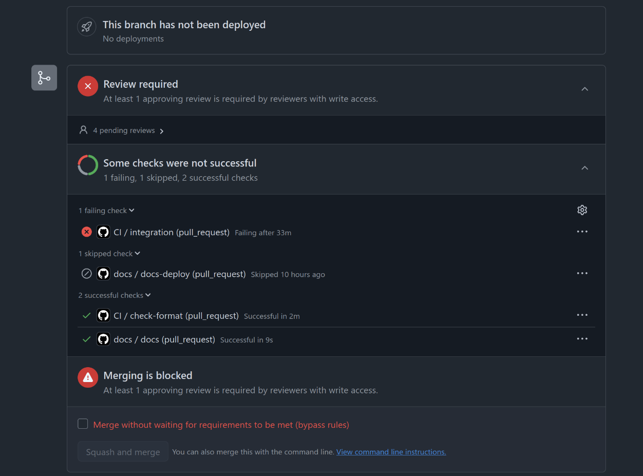
Click on any of the jobs to see more details. There, you can see the outcome of any individual step (as well as the console output).
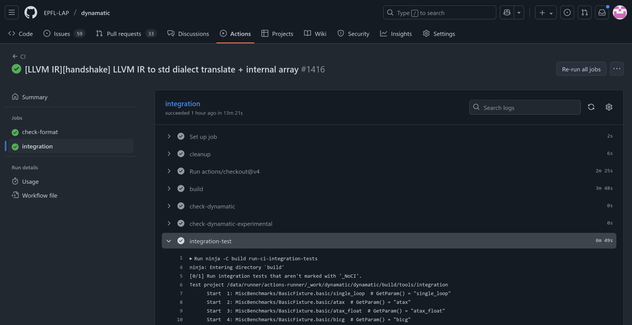
Files generated by integration tests (Dynamatic shell output, MLIR intermediate compilation results, HDL files, simulation logs…) are archived by the CI and uploaded to GitHub as an artifact. You can navigate to the workflow summary, where you can find and download the artifact at the bottom:
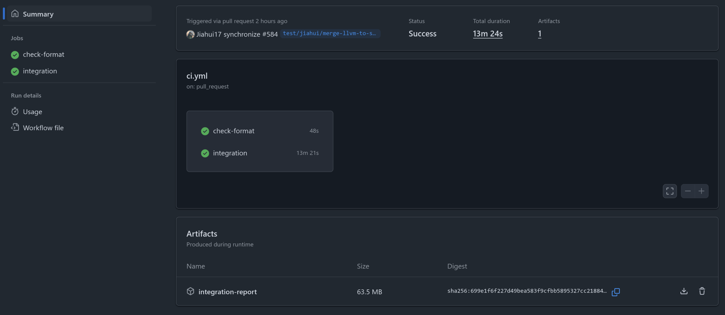
A new feature is the performance report. Integration test performance (in terms of cycles during the simulation) is collected and outputted in the form of a Markdown table. It is also located in the summary tab and looks like this:
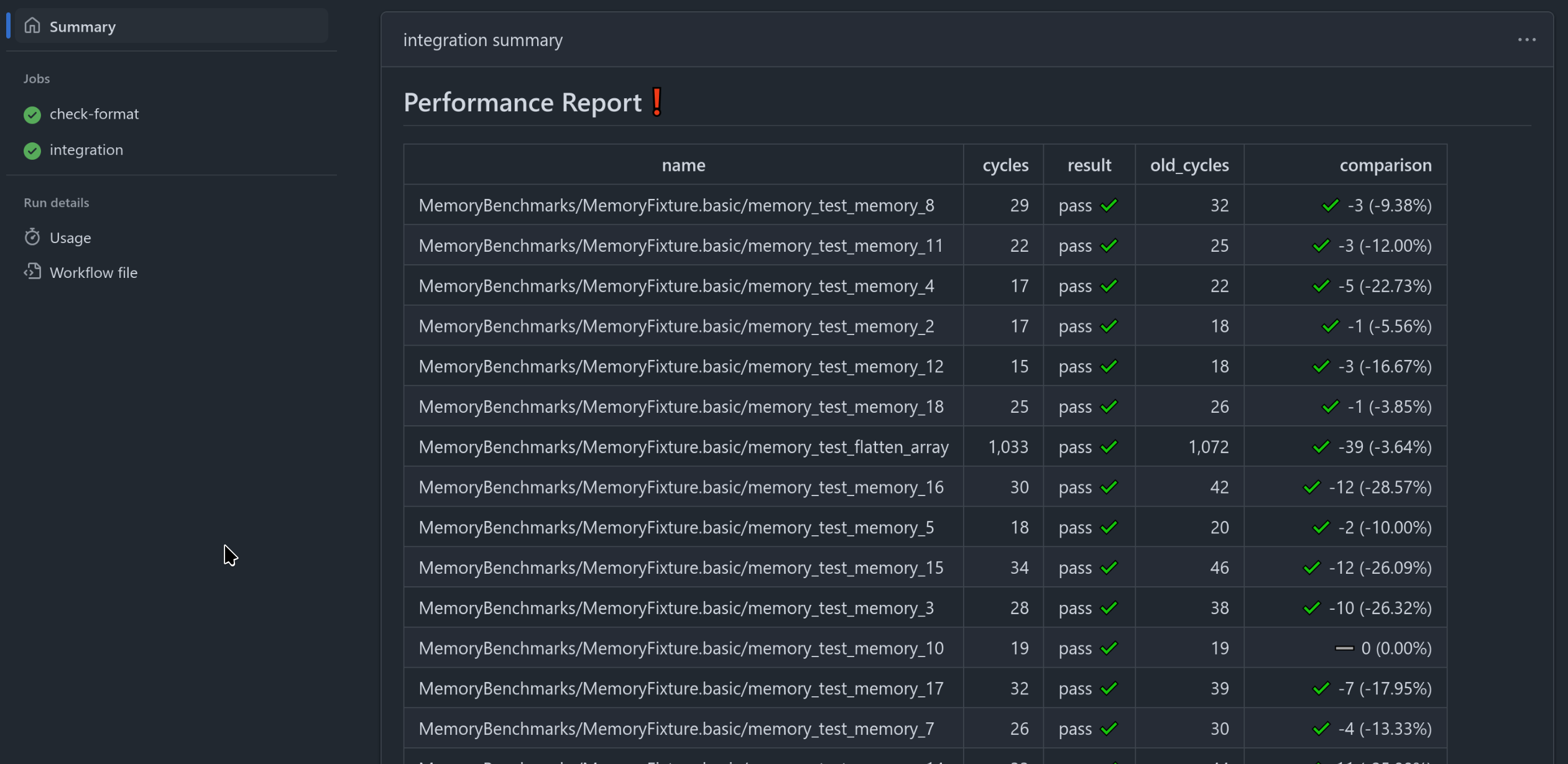
The performance report is generated by the Python script tools/integration/generate_perf_report.py. It works by picking up all cycle performances that were recorded during the integration test run and converting them to a user friendly tabular format. Internally, the script uses JSON representation for the performance report, which can easily be saved and parsed again. This is useful because the runner must keep track of what the performance of the main branch is, in order to compare all other branches to it. When a pull request is merged, the performance report saved on the runner is updated to match how the merged code performs. Also, the script will return a non-zero exit code if the worst performance difference compared to the previous report is worse than a given percentage. This percentage is set to 5% in the workflow (you can see the option --limit 5 that the script is called with in ci.yml).
The format of the report is the following. The cycles column is the performance of the current branch’s integration tests, while old_cycles is the performance that was last recorded in main. result is the outcome of the integration test. comparison is the difference cycles - old_cycles; positive is bad, negative is good. You can see the percent difference in the parentheses to the right. If any one test has a comparison percent value worse than 5%, the job will fail and you will have a red exclamation mark at the top notifying you that something is not right. Of course, you can always ignore this if you deem the performance difference to be insignificant.
FAQ
-
What OS does the self-hosted runner use?
- Ubuntu 24.04.2 LTS.
-
How do I install dependencies on the self-hosted runner?
- You can’t; ask someone who has access.
-
What are the “defaults” that the workflow runs?
- The basic integration tests run the following commands in
bin/dynamatic:set-dynamatic-path <DYNAMATIC_ROOT_FOLDER> set-src <PATH_TO_BENCHMARK> # e.g. integration-test/fir/fir.c` set-clock-period 5 compile --buffer-algorithm fpga20 write-hdl --hdl vhdl simulate exit
- The basic integration tests run the following commands in
-
How do I add a certain feature in the “default” verification flow? / How do I make it run with different flags (e.g. different buffering algorithms)?
- Add an integration test that runs whatever code you want the verification flow to run. Note that tests whose names contain the string
NoCIwill be ignored by the workflow. See Integration.
- Add an integration test that runs whatever code you want the verification flow to run. Note that tests whose names contain the string
-
How do I run the same thing that the CI does on my machine?
- For integration tests, use
ninja -C build run-ci-integration-tests. For formatting checks, see Formatting.
- For integration tests, use
-
The CI is failing the formatting check, but it passes it on my machine, what’s wrong?
- Make sure you have the same version of clang-format and autopep8 as the ones used in the CI. You can see which versions are used in the
.github/workflows/ci.ymlfiles.
- Make sure you have the same version of clang-format and autopep8 as the ones used in the CI. You can see which versions are used in the
-
Is there a possibility of leftover state from previous runs to affect my run on the self-hosted runner?
- No. This used to be a problem, but in the current setup, the entire workspace folder is emptied before the
integrationjob runs. The only thing that is shared is ccache’s cache, which is located somewhere else on the runner. This is because without it, building Polygeist would take a very very long time. We trust that ccache does its job properly, but if you are certain that it is the culprit for some issue you are having, contact someone with runner access to clear the cache for you.
- No. This used to be a problem, but in the current setup, the entire workspace folder is emptied before the
Backend
This document provides an overview of the current system used to transform the external modules of the Hardware IR into concrete RTL units. (More information about the Hardware IR can be found in the full backend documentation).
How we emit the RTL units is far from a complete, finished product, but we here detail the reasons behind each decision, including both positive and negative consequences.
How Dynamatic Calls the Beta Backend
Background
To use the beta backend requires knowledge of some aspects of how Dynamatic compiles from the Handshake IR down to RTL, and so this is first discussed:
Handshake IR
In the Handshake IR, there are many types of operations, declared in HandshakeOps.td or HandshakeArithOps.td. These operations become C++ classes, which provide many useful member functions and member variables. Each operation defines how it can be added to the IR (through MLIR builders), as well how it should be verified (both its own member variables, as well as verification of its input operands and output results).
Each Handshake operation is fully self-contained: all information about the operation is stored in the operation, and the operation knows nothing about other operations.
Hardware IR
During compilation, the Handshake IR is lowered to the Hardware IR.
RTL languages are based on a pattern of “definition” and “instances”. The “definition” contains all information about an object in one place, and many “instances” can share this information by containing a reference to their corresponding definition.
The Hardware IR aims to replicate this pattern inside the MLIR eco-system. First, a definition is built for each Handshake operations. Then, if two (or more) operations have exactly identical definitions, their definitions are merged.
ModuleExternOp
Each definition is added to the Hardware IR as a HWModuleExternOp(declared in HWStructure.td), an operation with no inputs or outputs. Any information needed to generate the RTL is stored in this operation, and it can be referenced by multiple instances.
InstanceOp
Each original Handshake operation is considered an instance, and so is converted to an InstanceOp, (also declared in HWStructure.td) a generic, (mostly empty) C++ class. Each InstanceOp has a reference to the corresponding HWModuleExternOp.
This means, in contrast to the Handshake IR, the Hardware IR does not use different C++ classes to represent different operations. There is very little functionality present to analyze or alter the Hardware IR once generated.
Each InstanceOp contains only 3 pieces of information: 1) its unique name, 2) a reference to a HWExternalModuleOp, 3) the names of its inputs and outputs.
Example
Below the serialized representation of a ConstantOp can be seen for both Handshake and Hardware.
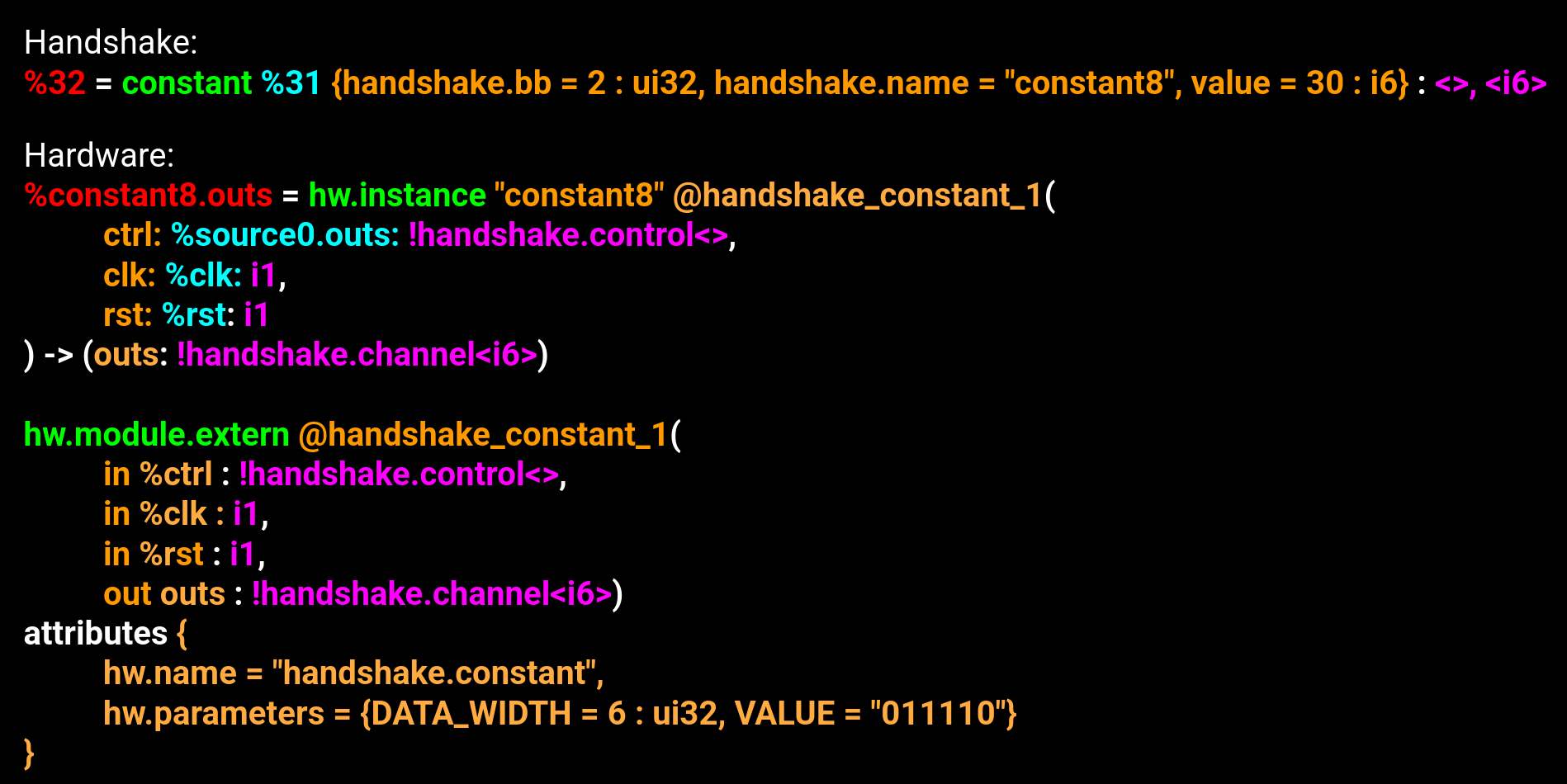
The output of the operation is highlighted in red. The inputs to the operation are highlighted in blue. The C++ class of the operation is highlighted in green. The information the operation contains is highlighted in orange. The type information of the inputs and outputs is highlighted in pink.
In the Handshake IR, the ConstantOp contains value = 30 : i6, which indicates the value of the constant is a 6-bit integer of value 30.
In the Hardware IR, the InstanceOp representing this constant instead has a reference to @hardware_constant_1. While all information about the inputs and outputs is present, there is no information about the operation itself (include what type of operation it is).
The HWModuleExternOp first contains the value used to reference it, in this case, @handshake_constant_1. It then redundantly contains all the input and output name and type information (as this information is also present on all the instances). Finally, after the attributes keywrod, it contains the information shared between the instances which they are missing: in this case, their original operation type (handshake.constant), (redundantly) the constant bitwidth (6), as well as the constant value ("011110")
Value
The usefulness of the Hardware IR is unclear: if we simply generated a unique definition for every single Handshake operation, the RTL files would be larger, but the final circuits would be the same. The Hardware IR is serialized very differently to the Handshake IR, which can make them annoying to compare.
While important memory system details are handled in the conversion between Handshake and Hardware, the fact that the printed IR is 1) not alterable or analyzable programatically due to the conversion to InstanceOp, and 2) annoying to read, means that its existance as an IR will probably be removed eventually.
Step 1: Merging Definitions
The first relevant part of compilation is the process of generating HWModuleExternOp from all the HandshakeOps. The relevant piece of code is:
https://github.com/EPFL-LAP/dynamatic/blob/aa984a5925706e19fe718cabc05c9874e679dd39/lib/Conversion/HandshakeToHW/HandshakeToHW.cpp#L545-L561
An if statement checks for each type of Handshake operation, and from it builds a dictionary representing the definition. This dictionary will be stored directly on the HWModuleExternOp, and a HWModuleExternOp is generated for each unique dictionary.
Any value which affects if two Handshake operations should share a HWModuleExternOp should be placed in this dictionary inside this if statement.
Step 2: Additional Information for Generation
The dictionary used to define a HWModuleExternOp was not designed with the beta backend in mind, and is unsuitable for directly making RTL generation decisions. This is mainly based on serialization approaches: while the C++ dictionary can contain complex C++ objects, the RTL generation decisions must be encoded as strings.
For this reason, a second set of if statements exists, at:
https://github.com/EPFL-LAP/dynamatic/blob/aa984a5925706e19fe718cabc05c9874e679dd39/lib/Support/RTL/RTL.cpp#L284-L291
These if statements are analysis ran on the Hardware IR, which as discussed above cannot really by analyzed. They are therefore extremely fragile. However, they were placed here to minize impact on the default backend during development.
The second set of if statements analyzes the HWModuleExternOp dictionary to better format the information for RTL generation. This helps with the goal of keeping the RTL generation as simple as possible: analysis is done on the IR, the beta backend is simply text manipulation.
Step 3: JSON Files for Parameter Passing
A json file controls how information passes from the C++ MLIR-based flow to the python text printing logic.
As discussed in the backend documentation, the JSON file is relatively powerful. The beta backend uses very few of its features, as it is not quite powerful enough, but this means the syntax can be complex.
An example entry is:
  {
    "name": "handshake.addf",
    "parameters": [
      {
        "name": "LATENCY",
        "type": "unsigned"
      },
      {
        "name": "INTERNAL_DELAY",
        "type": "string"
      },
      {
        "name": "FPU_IMPL",
        "type": "string"
      }
    ],
    "generator": "python $DYNAMATIC/experimental/tools/unit-generators/vhdl/vhdl-unit-generator.py -n $MODULE_NAME -o $OUTPUT_DIR/$MODULE_NAME.vhd -t addf -p is_double=$IS_DOUBLE fpu_impl='\"$FPU_IMPL\"' internal_delay='\"$INTERNAL_DELAY\"' latency=$LATENCY extra_signals=$EXTRA_SIGNALS",
    "dependencies": [
      "flopoco_ip_cores", "vivado_ip_wrappers"
    ]
  },
  {
    "name": "second_dependency",
    "generic": "/path/to/second/dependency.vhd",
  }
]
At the moment the dependency management system is relatively barebone; only parameter-less components can appear in dependencies since there is no existing mechanism to transfer the original component’s parameters to the component it depends on (therefore, any dependency with at least one parameter will fail to match due to the lack of parameters provided during dependency resolution, see matching logic).
module-name
note
The module-name option supports parameter substitution.
During RTL emission, the backend associates a module name to each RTL component concretization to uniquely identify it with respect to
- differently named RTL components, and to
- other concretizations of the same RTL component with different RTL parameter values.
By default, the backend derives a unique module name for each concretization using the following logic.
- For generic components, the module name is set to be the filename part of the filepath, without the file extension. For the example given in the generic section which associates the string
$DYNAMATIC/data/vhdl/handshake/mux.vhdto thegenerickey, the derived module name would simply bemux. - For generated components, the module name is provided by the backend logic itself, and is in general derived from the specific RTL parameter values associated to the concretization.
The MODULE_NAME backend parameter stores, for each component concretization, the associated module name. This allows JSON values supporting parameter substitution to include the name of the RTL module they are expected to generate during concretization.
warning
The backend uses module names to determine whether different component concretizations should be identical. When an RTL component is selected for concretization and the derived module name is identical to a previously concretized component, then the current component will be assumed to be identical to the previous one and therefore will not be concretized anew. This makes sense when considering that each module name indicates the actual name of the RTL module (Verilog module keyword or VHDL entity keyword) that the backend expects the concretization step to bring into the “current workspace” (i.e., to implement in a file inside the output directory). Multiple modules with the same name would cause name clashes, making the resulting RTL ambiguous.
The module-name, when present, must map to a string which overrides the default module name for the component. In the following example, the generic handshake.mux component would normally get asssigned the mux module name by default, but if the actual RTL module inside the file was named a_different_mux_name we could indicate this using the option as follows (some JSON content omitted for brevity).
{
  "name": "handshake.mux",
  "generic": "$DYNAMATIC/data/vhdl/handshake/mux.vhd",
  "module-name": "a_different_mux_name"
}
arch-name
note
The arch-name option supports parameter substitution.
The internal implementation of VHDL entities is contained in so-called “architectures”. Because there may be multiple such architectures for a single entity, each of them maps to a unique name inside the VHDL implementation. Instantiating a VHDL entitiy requires that one specifies the chosen architecure by name in addition to the entity name itself. By default, the backend assumes that the architecture to choose when instantiating VHDL entities is called “arch”.
The arch-name option, when present, must map to a string which overrides the default architecture name for the component. If the architecture of our usual handshake.mux example was named a_different_arch_name then we could indicate this using the option as follow (some JSON content omitted for brevity).
{
  "name": "handshake.mux",
  "generic": "$DYNAMATIC/data/vhdl/handshake/mux.vhd",
  "arch-name": "a_different_arch_name"
}
IMPORTANT: To support this feature also in Veriloge where multiple architectures of the same module can coexist, we use this parameter to select the desired architecture. This parameter effectively replaces the module name, allowing each architecture variant to be treated as a distinct module. For example, when generating a floating-point adder with three pipeline stages—whose structure differs from versions with other pipeline depths—we use the architecture’s name as the module name. Consequently, this architecture name must match the module name defined in the corresponding Verilog file.
use-json-config
note
The use-json-config option supports parameter substitution.
When an RTL component is very complex and/or heavily parameterized (e.g., the LSQ), it may be cumbersome or impossible to specify all of its parameters using our rather simple RTL typed parameter system. Such components may provide the use-json-config option which, when present, must map to a string indicating the path to a file in which the backend can JSON-serialize all RTL parameters associated to the concretization. This file can then be deserialized from a component generator to get back all generation parameters easily. Consequentlt, this option does not really make sense for generic components.
Below is an example of how you would use such a parameter for generating an LSQ by first having the backend serialize all its RTL parameters to a JSON file.
{
  "name": "handshake.lsq",
  "generic": "/my/lsq/generator --config \"$OUTPUT_DIR/$MODULE_NAME.json\"",
  "use-json-config": "$OUTPUT_DIR/$MODULE_NAME.json"
}
hdl
The hdl option, when present, must map to a string indicating the hardware description language (HDL) in which the concretized component is written. Possible values are vhdl (default), or verilog. If the handshake.mux component was written in Verilog, we would explictly specify it as follows.
{
  "name": "handshake.mux",
  "generic": "$DYNAMATIC/data/vhdl/handshake/mux.vhd",
  "hdl": "verilog"
}
io-kind
The io-kind option, when present, must map to a string indicating the naming convention to use for the module’s ports that logically belong to arrays of bitvectors. This matters when instantiating the associated RTL component because the backend must know how to name each of the individual bitvectors to do the port mapping.
- Generic RTL modules may have to use something akin to an array of bitvectors to represent such variable-sized ports. In this case, each individual bitvector’s name will be formed from the base port name and a numeric index into the array it represents. This
io-kindis calledhierarchical(default). - RTL generators, like Chisel, may flatten such arrays into separate bitvectors. In this case, each individual bitvector’s name will be formed from the base port name along with a textual suffix indicating the logical port index. This
io-kindis calledflat.
Let’s take the example of a multiplexer implementation with a configurable number of data inputs. Its VHDL implementation could follow any of the two conventions.
With hierarchical IO, the component’s JSON description (some content omitted for brevity) and RTL implementation would look like the following.
{
  "name": "handshake.mux",
  "generic": "$DYNAMATIC/data/vhdl/handshake/mux.vhd",
  "io-kind": "hierarchical"
}
entity mux is
  generic (SIZE : integer; DATA_WIDTH : integer);
  ports (
    -- all other IO omitted for brevity
    dataInputs : in array(SIZE) of std_logic_vector(DATA_WIDTH - 1 downto 0)
  );
end entity;
This entry matches to the AddFOp op based on the name field.
The three parameters are values from the HWModuleExternOp dictionary. The JSON files allows different RTL generation methods to be “matched with” based on the values in the dictionary. Adding these 3 parameters enforces that every AddFOp contains these values in their dictionaries for generation, and therefore allows us to pass these values to the python script.
There are parameters in the python call that is not in the parameters JSON field. One example is is_double. This value is not in the HWModuleExternOp dictionary, but was added as further analysis in the second set of if statements, ran on the Hardware IR. Since it is not in the original dictionary, we do not need to “match with” it.
Analysis of How Dynamatic Calls the Beta Backend
This system is very, very messy. Two sets of if statements, JSON matching based on the parameters in the first dictionary but not on the second, analysis on the Hardware IR: these should all be removed.
This is primarily due to Dynamatic’s original backend foreseeing that it would generate a lot of the simple units internally, and only generate complex units externally.
However, systems like speculation and taint tracking means that even simple units can have complex RTL generation. There are many many features in the original backend we no longer use, as while they are powerful, they do not give 100% of the functionality required. However, their existance makes the process more complex. The presence of the Hardware IR itself also makes this process more complex.
While pivoting from the Hardware IR is not possible in the immediate future, the goal is to remove both sets of if statements, and the JSON file, relatively soon. Instead interfaces will be used such that each Handshake operation has its own code to build its (correctly serialized) HWModuleExternOp dictionary.
The Beta Backend
The majority of the Beta Backend is very simple: it prints RTL code which is only lightly parameterized.
There are three aspects worth discussing:
Signal Managers
Speculation. taint tracking, and tagged tokens for multi-threading, require wrappers around core RTL units to deal with tokens that contain more than one payload. These are discussed in detail here.
Dependency Management
To avoid communication between the generators of each unit, each unit generates its own dependencies. This means there are many copies of common dependencies, such as joins and forks.
Arithmetic Units with IP cores
For arithmetic units which have IP cores, the beta backend does not handle the IP cores themselves: these are generated offline, and imported into the synthesis or simulation library unconditonally.
However, the beta backend does generate the following wrapper, which is mostly IP agnostic:
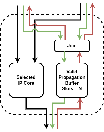
To generate the wrapper, the beta backend needs 2 pieces of information: 1) which ip core to use, and 2) how many slots to place in the valid propagation buffer.
Our IP selection system is both relatively new and imperfect: currently the beta backend may combine several parameters to select an IP core. In future, this should be changed so the entire IP core name is simply passed to the beta backend.
Full Backend Features
note
This document describes all features of the C++ backend of Dynamatic. While all of these features are still present in Dynamatic, many are no longer used: the dependency system, generics, and parameter-based matching should all be considered ‘to depreciate’.
This document describes the interconnected behavior of our RTL backend and of the JSON-formatted RTL configuration file, which together bridge the gap between MLIR and synthesizable RTL. There are two main sections in this document.
- Design | Provides an overview of the backend’s design and its underlying rationale.
- RTL configuration | Describes the expected JSON format for RTL configuration files.
- Matching logic | Explains the logic that the backend uses to parse the configuration file and determine the mapping between MLIR and RTL.
Design
The RTL backend’s role is to transform a semi-abstract in-MLIR representation of a dataflow circuit into a specific RTL implementation that matches the behavior that the IR expresses. As such, the backend does not alter the semantics of its input circuit; rather, its task is two-fold.
- To emit synthesizable RTL modules that implement each operation of the input IR.
- To emit the “glue” RTL that connects all the RTL modules together to implement the entire circuit.
The first subtask is by far the most complex to implement in a flexible and robust way, whereas the second subtask is easily achievable once we know how to instantiate each of the RTL module we need. As such this design section heavily focuses on how our RTL backend fulfills the first one’s requirements. The next section indirectly touches on both subtasks by describing how RTL configuration files dictate RTL emission.
Formally, the RTL backend is a sequence of two transformations handled by two separate binaries. This process’s starting point is the fully optimized and buffered Handshake-level IR produced by our numerous transformation and optimization passes.
- In a first step, Handshake operations are converted to HW (read “hardware”) operations; HW is a “lower-level” MLIR dialect whose structure closely ressembles that of RTL code. This is achieved by running the
HandshakeToHWconversion pass using Dynamatic’s optimizer (dynamatic-opt). In addition to performing the lowering of Handshake operations, the conversion pass also adds information to the IR that tells the second step which standard RTL modules the circuit uses. - In the second step, the HW-level IR emitted by the first step goes through our RTL emitter (
export-vhdl), which produces synthesizable RTL.
Handshake to HW
The HandshakeToHW conversion pass may appear unnecessary at first glance; one could imagine going directly from Handshake-level IR to RTL without any intermediate IR transformation. While this would certainly be possible, we argue that the resulting backend would become quite complex for no discernable advantage. Having the conversion pass as a kind of pre-processing step to the actual RTL emission allow us to separate concerns in an elegant way, yielding two manageable pieces of software that, while intrinsically linked, are technically independent.
In particular, the conversion pass offloads multiple IR analysis/transformation steps from the RTL emission logic and is able to emit a valid (HW-level) IR that showcases the result of these transformations in a convenient way. The ability to observe the close-to-RTL in-MLIR representation of the circuit before emitting the actual RTL makes debugging significantly easier, as one can see precisely what circuit will be emitted (identical IO ports, module names, etc.); this would be impossible or at least cumbersome had these transformations happened purely in-memory. Importantly, the conversion pass
- makes memory interfaces (i.e., their respective signal bundle in the top-level RTL module) explicit,
- identifies precisely the set of standard RTL modules we will need in the final circuit, and
- associate a port name to each SSA value use and each SSA result and store it inside the IR to make the RTL emitter’s job as minimal as possible.
Making memory interfaces explicit
IR at the Handshake level still links MLIR operations representing memory interfaces (e.g., LSQ) inside dataflow circuits to their (implicitly represented) backing memories using the standard mlir::MemRefType type, which abstracts the underlying IO that will eventually connect the two together. For example, a Handshake function operating on a single 32-bit-wide integer array of size 64 has the following signature (control signals omitted).
handshake.func @func(%mem: memref<64xi32>) -> none { ... }
The conversion pass would lower this Handshake function (handshake::FuncOp) to an equivalent HW module (hw::HwModuleOp) with a signature that makes all the signals connecting the memory interface to its memory explicit (the following snippet omits control signals for brevity).
hw.module @func(in %mem_loadData : i32, out mem_loadEn : i1, out mem_loadAddr : i32,
                out mem_storeEn : i1, out mem_storeAddr : i32, out mem_storeData : i32) { ... }
note
Note that unlike in the Handshake function, the HW module’s inputs and outputs are between parentheses.
The single memref-typed mem argument to the Handshake function is replaced by one module input (mem_loadData) and 5 module outputs (mem_loadEn, mem_loadAddr, mem_storeEn, mem_storeAddr, and mem_storeData) that all have simple types immediately lowerable to RTL. The interface’s actual specification (i.e., the composition of the signal bundle that the memref lowers to) is a separate concern; shown here is Dynamatic’s current memory interface, but it could in practice be any signal bundle that fits one’s needs.
Identifying necessary modules
In the general case, every MLIR operation inside a Handshake function in the input IR ends up being emitted as an instantiation of a specific RTL module. The mapping between these MLIR operations and the eventual RTL instantiations being one-to-one, this part of the conversion is relatively trivial to implement and think about. One less trivial matter, however, is determining what those instances should be of. In other words, which RTL modules need to be instantiated and therefore need be part of the final RTL design.
Consider the following handshake::MuxOp operation, which represents a regular dataflow multiplexer taking any strictly positive number of data inputs and a select input to dictate which of the data inputs should be forwarded to the single output.
%result1 = handshake.mux %select [%data1, %data2] : i1, i32
This particular multiplexer has 2 data inputs whose data bus is 32-bit wide, and a 1-bit wide select input (1 bit is enough to select between 2 inputs). Now consider this second multiplexer which, despite having the same identified characteristics, has different data inputs.
// Previous multipexer
%result1 = handshake.mux %select [%data1, %data2] : i1, i32

// New one with same characteristics
// - 2 data inputs
// - 32-bit data bus
// - 1-bit select bus
%result2 = handshake.mux %select [%data3, %data4] : i1, i32
As mentioned before, each of these two multiplexers would be emitted as a separate instantiation of a specific RTL module. However, it remains to determine whether these two instantiations would be of the same RTL module. In that particular example, both multiplexer modules (whether they were different or identical) would have the same top-level IO. Indeed, the three characteristics we previously identified (number of data inputs, data bus width, select bus width) completely characterize the multiplexer’s RTL interface (their gate-level implementation could of course be different).
Predictably, not all multiplexers will have the same RTL interface. Consider the following multiplexer with 16-bit data buses.
// Previous multipexers with
// - 2 data inputs
// - 32-bit data bus
// - 1-bit select bus
%result1 = handshake.mux %select [%data1, %data2] : i1, i32
%result2 = handshake.mux %select [%data3, %data4] : i1, i32

// This multiplexer has 16-bit data buses instead of 32
%result3 = handshake.mux %select [%data5, %data6] : i1, i16
It should be clear that there is not, at least in the general case, a clear correspondance between Handshake operation types (e.g., handshake::MuxOp) and the interface of the RTL module they will eventually being emitted as. Two MLIR operations of the same type may be emitted as two RTL instances of the same RTL module, or as two RTL instances of different RTL modules. The conversion pass needs a way to identify its concrete RTL module needs based on its input IR.
We introduce the concept of RTL parameter to formalize this mapping between MLIR operations and RTL modules. The general idea is, during conversion of each Handshake-level MLIR operation to an hw::InstanceOp—the HW dialect’s operation that represents RTL instances—to identify the “intrinsic structural characteristics” of each operation and add to the IR an operation that will instruct the RTL emitter to emit a matching RTL module. We call these “intrinsic structural characteristics” RTL parameters, and we encode them as attributes to hw::HWModuleExternOp operations, which as their name suggest represent external RTL modules that are needed by the main module’s implementation.
Consider an input Handshake function containing the three multiplexers we previously described (all other operations omitted).
handshake.func @func(...) -> ... {
  ...
  // 2 data inputs, 32-bit data, 1-bit select
  %result1 = handshake.mux %select [%data1, %data2] : i1, i32
  %result2 = handshake.mux %select [%data3, %data4] : i1, i32
  // 2 data inputs, 16-bit data, 1-bit select
  %result3 = handshake.mux %select [%data5, %data6] : i1, i16
  ...
}
The conversion pass would lower this Handshake function to something that looks like the following (details omitted for brevity).
// RTL module directly corresponding to the input Handshake function.
// This is the "glue" RTL that connects everything together.
hw.module @func(...) {
  ...
  // 2 data inputs, **32-bit data**, 1-bit select
  %result1 = hw.instance @mux_32 "mux1" (%select, %data1, %data2) -> channel<i32>
  %result1 = hw.instance @mux_32 "mux2" (%select, %data3, %data4) -> channel<i32>

  // 2 data inputs, **16-bit data**, 1-bit select
  %result1 = hw.instance @mux_16 "mux3" (%select, %data5, %data6) -> channel<i16>
  ...
}

// RTL module corresponding to the mux variant with **32-bit data**.
// The RTL emitter will need to *concretize* an RTL implementation for this module.
hw.module.extern @mux_32( in channel<i1>, in channel<i32>,
                          in channel<i32>, out channel<i32>) attributes {
  hw.name = "handshake.mux",
  hw.parameters = {SIZE = 2 : ui32, DATA_WIDTH = 32 : ui32, SELECT_WIDTH = 1 : ui32}
}


// RTL module corresponding to the mux variant with **16-bit data**.
// The RTL emitter will need to *concretize* an RTL implementation for this module.
hw.module.extern @mux_16( in channel<i1>, in channel<i16>,
                          in channel<i16>, out channel<i16>) attributes {
  hw.name = "handshake.mux",
  hw.parameters = {SIZE = 2 : ui32, DATA_WIDTH = 16 : ui32, SELECT_WIDTH = 1 : ui32}
}
Observe that while each multiplexer maps directly to a hw.instance (hw::InstanceOp) operation, the conversion pass only produces two external RTL modules (hw.module.extern): one for the multiplexer variant with 32-bit data, and one for the variant with 16-bit data. These hw.module.extern (hw::HWModuleExternOp) operations encode two important pieces of information in dedicated MLIR attributes.
hw.nameis the canonical name of the MLIR operation from which the RTL module originates, here the Handshake-level multiplexerhandshake.mux.hw.parametersis a dictionary mapping each of the multiplexers’s RTL parameter to a specific value.
Importantly, each input operation type defines the set of RTL parameters which characterizes it. As we just saw, for multiplexers these are the number of data inputs (SIZE), the data-bus width (DATA_WIDTH), and the select-bus width (SELECT_WIDTH). The conversion pass will generate one external module definition for each unique combination of RTL name and parameter values dervied from the input IR. These are the RTL modules that the second part of the backend, the RTL emitter, will need to derive an implementation for so that they can be instantiated from the main RTL module. We call this step concretization and explain its underlying logic in the RTL emission subsection.
important
While the pass itself sets RTL parameters purely according to each operation’s structural characteristics, nothing prevents passes up the pipeline to already set arbitrary RTL parameters on MLIR operations. The HandshakeToHW conversion pass treats RTL parameters already present in the input IR transparently by considering them on the same level as the structural parameters it itself sets (unless there is a name conflict, in which case it emits a warning). It is then up to the backend’s RTL configuration to recognize these “extra RTL parameters” and act accordingly (they may be ignored if nothing is done, resulting in a “regular” RTL module being concretized, see the matching logic). For example, a pass up the pipeline may wish to distinguish between two different RTL implementations (say, A and B) of handshake.mux operations in order to gain performance. Such a pass could already tag these operations with an RTL parameter (e.g., hw.parameters = {IMPLEMENTATION = "A"}) to carry that information down the pipeline and, with proper support in the backend’s RTL configuration, concretize and instantiate the intended RTL module.
Port names
At the Handshake level, the input and output ports of MLIR operations (in MLIR jargon, their operands and results) do not have names. In keeping with the objective of the HandshakeToHW conversion pass to lower the IR to a close-to-RTL representation, the pass associates a port name to each input and output port of each HW-level instance and (external) module operation. These port names will end up as-is in the emitted RTL design (unless explicitly modified by the RTL configuration, see JSON options io-kind, io-signals, and io-map). They are derived through a mix of means depending on the specific input MLIR operation type.
warning
The port names and their ordering influences the experimental backend that uses python generators, so if any changes are needed they should be reflected also in the generators. Special attention should be given to the relative order of data and valid signal implemented in the export-rtl.cpp.
RTL emission
The RTL emitter picks up the IR that comes out of the HandshakeToHW conversion pass and turns it into a synthesizable RTL design. Importantly, the emitter takes as additional argument a list of JSON-formatted RTL configuration files which describe the set of parameterized RTL components it can conretize and instantiate; the next section covers in details the configuration file’s expected syntax, including all of its options.
After parsing RTL configuration files, the emitter attempts to match each hw.module.extern (hw::HWModuleExternOp) operation in its input IR to entries in the configuration files using the hw.name and hw.parameters attributes; the last section describes the matching logic in details. If a matching RTL component is found, then the emitter concretizes the RTL module implementation that corresponds to the hw.module.extern operation into the final RTL design. This concretization may be as simple as copying a generic RTL implementation of a component to the output directory, or require running an arbitrarily complex RTL generator that will generate a specific implementation of the component that depends on the specific RTL parameter values. RTL configuration files dictate the concretization method for each RTL component they declare. If any hw.module.extern operation finds no match in the RTL configuration, RTL emission fails.
Circling back to the multiplexer example, it is possible to define a single generic RTL multiplexer implementation that is able to implement all possible combinations of RTL parameter values. Assuming an appropriate RTL configuration, the RTL emitter would simply copy that known generic RTL implementation to the final RTL design if its input IR contained any hw.module.extern operation with name handshake.mux and valid value for each of the three RTL parameters.
Emitting each hw.module (hw::hwModuleOp) and hw.instance (hw::InstanceOp) operation to RTL is relatively straightforward once all external modules are concretized. This translation is almost one-to-one, requires little work, and is HDL-independent beyond syntactic concerns.
RTL configuration
An RTL configuration file is made up of a list of JSON objects which each describe a parameterized RTL component along with
- a method to retrieve a concrete implementation of the RTL component for each valid combination of parameters (a step we call concretization),
- a list of timing models for the component, each optionally constrained by specific RTL parameter values, and
- a list of options.
Component description format
Each JSON object describing an RTL component should specify a mandatory name key and optional parameters and models keys.
{
  "name": "<name-of-the-corresponding-mlir-op>",
  "parameters": [],
  "models": []
}
- The
namekey must map to a string that identifies the RTL component the entry corresponds to. For RTL components mapping one-to-one with an MLIR operation, this would typically be the canonical MLIR operation name. For example. for a mux it would behandshake.mux. - The
parameterskey must map to a list of JSON objects, each describing a parameter of the RTL component one must provide to derive a concrete implementation of the component. For example, for a mux these parameters would be the number of data inputs (SIZE), the data bus width on all data inputs (DATA_WIDTH), and the data bus width of the select signal (SELECT_WIDTH). The “parametersformat” section describes the expected and recognized keys in each JSON object. If theparameterskey is omitted, it is assumed to be an empty list. - The
modelskey must map to a list of JSON objects, each containing the path to a file containing a timing model for the RTL component. RTL component parameters generally have an influence on a component’s timing model; therefore, it is often useful to specify multiple timing models for various combinations of parameters, along with a generic unconstrained fallback model to catch all remaining combinations. To support such behavior, each model in the list may optionally define constraints on the RTL parameters (using a similar syntax as during parameter description) to restrict the applicability of the model to specific conretizations of the component for which the constraints are verified. For example, for a mux we could have a specific timing model when the mux has exactly two data inputs (SIZE == 2) and control-only data inputs (DATA_WIDTH == 0), and a second fallback model for all remaining parameter combinations. The “modelsformat” section describes the expected and recognized keys in each JSON object. If themodelskey is omitted, it is assumed to be an empty list.
The mux example described above would look like the following in JSON.
{
  "name": "handshake.mux",
  "parameters": [
      { "name": "SIZE", "type": "unsigned", "lb": 2 },
      { "name": "DATA_WIDTH", "type": "unsigned", "ub": 64 },
      { "name": "SELECT_WIDTH", "type": "unsigned", "range": [1, 6] }
    ],
  "models": [
    {
      "constraints": [
        { "parameter": "SIZE", "eq": 2 },
        { "parameter": "DATA_WIDTH", "eq": 0 }
      ],
      "path": "/path/to/model/for/control-mux-with-2-inputs.sdf"
    },
    { "path": "/path/to/model/for/any-mux.sdf" }
  ]
}
Concretization methods
Finally, each RTL component description must indicate whether the component must be concretized simply by replacing generic entity parameters during instantiation (implying that the component already has a generic RTL implementation with the same number of parameters as declared in the JSON entry), or by generating the component on-demand for specific parameter values using an arbitray generator.
- For the former, one would define the
generickey, which must map to the filepath of the generic RTL implementation on disk. - For the latter, one would define the
generatorkey, which must map to a shell command that, when ran, creates the implementation of the component at a specific filesystem location.
Exactly one of the two keys must exist for any given component (i.e., a component is either a generic or generated on-demand).
important
The string value associated to the generic and generator key supports parameter substitution; if it contains the name of component parameters prefixed by a $ symbol (shell-like syntax), these will be replaced by explicit parameter values during component concretization. Additionally, the backend provides a couple extra backend parameters during component concretization which hold meta-information useful during generation but not linked to any component’s specific implementation. Backend parameters have reserved names and are substituted with explicit values just like regular component parameters. The “special parameters” section lists all special parameters.
Parameter substitution is key for generated components, whose shell command must contain the explicit parameter values to generate the matching RTL implementation on request, but is often useful in other contexts too. When the backend supports parameter substitution for a particular JSON field, we explicitly indicate it in this specification.
Generic
If the mux were to be defined generically, the JSON would look like the following (parameters and models values ommited for brevity).
{
  "name": "handshake.mux",
  "generic": "$DYNAMATIC/data/vhdl/handshake/mux.vhd"
}
When concretizing a generic component, the backend simply needs to copy and paste the generic implementation into the final RTL design. During component instantiation, explicit parameter values are provided for each instance of the generic component, in the order in which they are defined in the parameters key-value pair. Note that $DYNAMATIC is a backend parameter which indicates the path to Dynamatic’s top-level directory.
Generator
If the mux needed to be generated for each parameter combination, the JSON would look like the following (parameters and models values ommited for brevity).
{
  "name": "handshake.mux",
  "generator": "/path/to/mux/generator $SIZE $DATA_WIDTH $SELECT_WIDTH --output \"$OUTPUT_DIR\" --name $MODULE_NAME"
}
When concretizing a generated component, the backend opaquely issues the provided shell command, replacing known parameter names prefixed by $ with their actual values (e.g., for the mux, $SIZE, $DATA_WIDTH, and $SELECT_WIDTH would be replaced by their corresponding parameter values). Note that $OUTPUT_DIR and $MODULE_NAME are backend parameters which indicate, respectively, the path to the directory where the generator must create a file containing the component’s RTL implementation, and the name of the main RTL module that the backend expects the generator to create.
Per-parameter concretization method
In some situations, it may be desirable to override the backend’s concretization-method-dependent behavior on a per-parameter basis. For example, specific RTL parameters of a generic component may be useful for matching purposes (see matching logic) but absent in the generic implementation of the RTL module. Conversely, a component generator may produce “partially generic” RTL modules requiring specific RTL parameters during instantiation.
All parameters support the generic key which, when present, must map to a boolean indicating whether the parameter should be provided as a generic parameter to instances of the concretized RTL module, regardless of the component’s concretization method. The backend follows the behavior dictated by the component’s concretization method for all RTL parameters that do not specify the generic key.
parameters format
Each JSON object describing an RTL component parameter must contain two mandatory keys.
{
  "parameters": [
    { "name": "<parameter-name>", "type": "<parameter-type>" },
    { "name": "<other-parameter-name>", "type": "<other-parameter-type>" },
  ]
}
- The
namekey must map to string that uniquely identifies the component parameter. Only alphanumeric characters, dashes, and underscores are allowed in parameter names. - The
typekey must map to a string denoting the parameter’s datatype. Currently supported values areunsignedfor an unsigned integer andstringfor an arbitrary sequence of characters.
Depending on the parameter type, additional key-value pairs constraining the set of allowed values are recognized.
unsigned
Unsigned parameters can be range-restricted (by default, any value greater than or equal to 0 is accepted) using the lb, ub, and range key-value pairs, which are all inclusive. Exact matches are possible using the eq key-value pair. Finally, ne allows to check for differences.
{
  "parameters": [
    { "name": "BETWEEN_2_AND_64", "type": "unsigned", "lb": 2, "ub": 64 },
    { "name": "SHORT_BETWEEN_2_AND_64", "type": "unsigned", "range": [2, 64] },
    { "name": "EXACTLY_4", "type": "unsigned", "eq": 4 },
    { "name": "DIFFERENT_THAN_2", "type": "unsigned", "ne": 2 },
  ]
}
string
For string parameters, only exact matches/differences are currently supported with eq and ne.
{
  "parameters": [
    { "name": "EXACTLY_MY_STRING", "type": "string", "eq": "MY_STRING" },
    { "name": "NOT_THIS_OTHER_STRING", "type": "string", "ne": "THIS_OTHER_STRING" },
  ]
}
Backend parameters
During component concretization, the backend injects extra backend parameters that are available for parameter substitution in addition to the parameters of the component being concretized. These parameters have reserved names which cannot be used by user-declared parameters in the RTL configuration file. All backend parameters are listed below.
DYNAMATIC: path to Dynamatic’s top-level directory (without a trailing slash).OUTPUT_DIR: path to output directory where the component is expected to be concretized (without a trailing slash). This is only really meaningful for generated components, for which it tells the generator the direcotry in which to create the VHDL (.vhd) or Verilog (.v) file containing the component’s RTL implementation. Generators can assume that the directory already exists.MODULE_NAME: RTL module name (or “entity” in VHDL jargon) that the backend will use to instantiate the component from RTL. Concretization must result in a module of this name being created inside the output directory. Since module names are unique within the context of each execution of the backend, generators may assume that they can create without conflict a file named$MODULE_NAME.<extension>inside the output directory to store the generated RTL implementation; in other words, a safe output path is"$OUTPUT_DIR/$MODULE_NAME.<extension>"(note the quotes around the path to handle potential spaces inside the output directory’s path correctly). This parameter is controllable from the RTL configuration file itsel, see the relevant option.
models format
Each JSON object describing a timing model must contain the path key, indicating the path to a timing model for the component.
{
  "models": [
    { "path": "/path/to/model.sdf" },
    { "path": "/path/to/other-model.sdf" },
  ]
}
Additionally, each object can contain the constraints key, which must map to a list of JSON objects describing a constraint on a specific component parameter which restricts the applicability of the timing model. The expected format matches closely that of the parameters array. Each entry in the list of constraints must reference a parameter name under the name key to denote the parameter being constrained. Then, for the associated parameter type, the same constraint-setting key-value pairs as during parameter definition are available to constrain the set of values for which the timing model should match.
The following example shows a component with two parameters and two timing models. One which restricts the set of possible values for both parameters, and an unconstrained fallback model which will be selected if the parameter values do not satisfy the first model’s constraints (components and concretization method fields ommited for brevity).
{
  "parameters": [
    { "name": "UNSIGNED_PARAM", "type": "unsigned" },
    { "name": "OTHER_UNSIGNED_PARAM", "type": "unsigned" },
    { "name": "STRING_PARAM", "type": "string" }
  ],
  "models": [
    {
      "constraints": [
        { "name": "UNSIGNED_PARAM", "lb": 4 },
        { "name": "STRING_PARAM", "eq": "THIS_STRING" },
      ],
      "path": "/path/to/model-with-constraints"
    },
    {
      "path": "/path/to/fallback/model.sdf"
    }
  ]
}
Options
Each RTL component description recognizes a number of options that may be helpful in certain situations. These each have a dedicated key name which must exist at the component description’s top-level and map to a JSON element of the valid type (depending on the specific option). See examples in each subsection.
dependencies
Components may indicate a list of other components they depend on (e.g., which define RTL module(s) that they instantiate within their own module’s implementation) via their name. When concretizing a component with dependencies, the backend will look for components within the RTL configuration whose name matches each of the dependencies and attempt to concretize them along the original component. The backend is able to recursively concretize dependencies’s dependencies and ensures that any dependency is concretized only a single time, even if it appears in the dependency list of multiple components in the current backend execution. This system allows to indirectly concretize “supporting” (i.e., depended on) RTL components used within the implementation of multiple “real” (i.e., corresponding to MLIR operations) RTL components seamlessly and without code duplication.
The dependencies option, when present, must map to a list of strings representing RTL component names within the configuration file. The list is assumed to be empty when omitted. In the following example, attempting to concretize the handshake.mux component will make the backend concretize the first_dependency and second_dependency components as well (some JSON content omitted for brevity).
[
  {
    "name": "handshake.mux",
    "generic": "$DYNAMATIC/data/vhdl/handshake/mux.vhd",
    "dependencies": ["first_dependency", "second_dependency"]
  },
  {
    "name": "first_dependency",
    "generic": "/path/to/first/dependency.vhd",
  },
  {
    "name": "second_dependency",
    "generic": "/path/to/second/dependency.vhd",
  }
]
At the moment the dependency management system is relatively barebone; only parameter-less components can appear in dependencies since there is no existing mechanism to transfer the original component’s parameters to the component it depends on (therefore, any dependency with at least one parameter will fail to match due to the lack of parameters provided during dependency resolution, see matching logic).
module-name
note
The module-name option supports parameter substitution.
During RTL emission, the backend associates a module name to each RTL component concretization to uniquely identify it with respect to
- differently named RTL components, and to
- other concretizations of the same RTL component with different RTL parameter values.
By default, the backend derives a unique module name for each concretization using the following logic.
- For generic components, the module name is set to be the filename part of the filepath, without the file extension. For the example given in the generic section which associates the string
$DYNAMATIC/data/vhdl/handshake/mux.vhdto thegenerickey, the derived module name would simply bemux. - For generated components, the module name is provided by the backend logic itself, and is in general derived from the specific RTL parameter values associated to the concretization.
The MODULE_NAME backend parameter stores, for each component concretization, the associated module name. This allows JSON values supporting parameter substitution to include the name of the RTL module they are expected to generate during concretization.
warning
The backend uses module names to determine whether different component concretizations should be identical. When an RTL component is selected for concretization and the derived module name is identical to a previously concretized component, then the current component will be assumed to be identical to the previous one and therefore will not be concretized anew. This makes sense when considering that each module name indicates the actual name of the RTL module (Verilog module keyword or VHDL entity keyword) that the backend expects the concretization step to bring into the “current workspace” (i.e., to implement in a file inside the output directory). Multiple modules with the same name would cause name clashes, making the resulting RTL ambiguous.
The module-name, when present, must map to a string which overrides the default module name for the component. In the following example, the generic handshake.mux component would normally get asssigned the mux module name by default, but if the actual RTL module inside the file was named a_different_mux_name we could indicate this using the option as follows (some JSON content omitted for brevity).
{
  "name": "handshake.mux",
  "generic": "$DYNAMATIC/data/vhdl/handshake/mux.vhd",
  "module-name": "a_different_mux_name"
}
arch-name
note
The arch-name option supports parameter substitution.
The internal implementation of VHDL entities is contained in so-called “architectures”. Because there may be multiple such architectures for a single entity, each of them maps to a unique name inside the VHDL implementation. Instantiating a VHDL entitiy requires that one specifies the chosen architecure by name in addition to the entity name itself. By default, the backend assumes that the architecture to choose when instantiating VHDL entities is called “arch”.
The arch-name option, when present, must map to a string which overrides the default architecture name for the component. If the architecture of our usual handshake.mux example was named a_different_arch_name then we could indicate this using the option as follow (some JSON content omitted for brevity).
{
  "name": "handshake.mux",
  "generic": "$DYNAMATIC/data/vhdl/handshake/mux.vhd",
  "arch-name": "a_different_arch_name"
}
use-json-config
note
The use-json-config option supports parameter substitution.
When an RTL component is very complex and/or heavily parameterized (e.g., the LSQ), it may be cumbersome or impossible to specify all of its parameters using our rather simple RTL typed parameter system. Such components may provide the use-json-config option which, when present, must map to a string indicating the path to a file in which the backend can JSON-serialize all RTL parameters associated to the concretization. This file can then be deserialized from a component generator to get back all generation parameters easily. Consequentlt, this option does not really make sense for generic components.
Below is an example of how you would use such a parameter for generating an LSQ by first having the backend serialize all its RTL parameters to a JSON file.
{
  "name": "handshake.lsq",
  "generic": "/my/lsq/generator --config \"$OUTPUT_DIR/$MODULE_NAME.json\"",
  "use-json-config": "$OUTPUT_DIR/$MODULE_NAME.json"
}
hdl
The hdl option, when present, must map to a string indicating the hardware description language (HDL) in which the concretized component is written. Possible values are vhdl (default), or verilog. If the handshake.mux component was written in Verilog, we would explictly specify it as follows.
{
  "name": "handshake.mux",
  "generic": "$DYNAMATIC/data/vhdl/handshake/mux.vhd",
  "hdl": "verilog"
}
io-kind
The io-kind option, when present, must map to a string indicating the naming convention to use for the module’s ports that logically belong to arrays of bitvectors. This matters when instantiating the associated RTL component because the backend must know how to name each of the individual bitvectors to do the port mapping.
- Generic RTL modules may have to use something akin to an array of bitvectors to represent such variable-sized ports. In this case, each individual bitvector’s name will be formed from the base port name and a numeric index into the array it represents. This
io-kindis calledhierarchical(default). - RTL generators, like Chisel, may flatten such arrays into separate bitvectors. In this case, each individual bitvector’s name will be formed from the base port name along with a textual suffix indicating the logical port index. This
io-kindis calledflat.
Let’s take the example of a multiplexer implementation with a configurable number of data inputs. Its VHDL implementation could follow any of the two conventions.
With hierarchical IO, the component’s JSON description (some content omitted for brevity) and RTL implementation would look like the following.
{
  "name": "handshake.mux",
  "generic": "$DYNAMATIC/data/vhdl/handshake/mux.vhd",
  "io-kind": "hierarchical"
}
entity mux is
  generic (SIZE : integer; DATA_WIDTH : integer);
  ports (
    -- all other IO omitted for brevity
    dataInputs : in array(SIZE) of std_logic_vector(DATA_WIDTH - 1 downto 0)
  );
end entity;
If we were to concretize a multiplexer with 2 inputs and 32-bit datawidth using the above generic component, we would need to name its data inputs dataInputs(0) and dataInputs(1) during instantiation. However, if we were to use a generator to concretize this specific multiplexer implementation, the component’s JSON description (some content omitted for brevity) and RTL implementation would most likely look like the following.
{
  "name": "handshake.mux",
  "generator": "/my/mux/generator $SIZE $DATA_WIDTH $SELECT_WIDTH",
  "io-kind": "flat"
}
entity mux is
  ports (
    -- all other IO omitted for brevity
    dataInputs_0 : in std_logic_vector(31 downto 0);
    dataInputs_1 : in std_logic_vector(31 downto 0)
  );
end entity;
We would need to name its data inputs dataInputs_0 and dataInputs_1 during instantiation in this case.
In both cases, the base name dataInputs is part of the specification of handshake.mux, the matching MLIR operation. Within the IR, these ports are always named following the flat convention: dataInputs_0 and dataInputs_1. During RTL emission, they will be converted to the first hierarchical form by default, or left as is if the io-kind is explicitly set to flat.
io-signals
The backend has naming convention when it comes to signals part of the same dataflow channel. By default, if the channel name is channel_name, then all signal names will start with the channel name and be suffixed by a specific (possibly empty) string.
- the data bus has no suffix (
channel_name), - the valid wire has a
_validsuffix (channel_name_valid), and - the ready wire has a
_readysuffix (channel_name_ready).
This matters when instantiating the associated RTL component because the backend must know how to name each of the individual signals to do the port mapping.
The io-signals option, when present, must map to a JSON object made up of key/string-value pairs where the key indicates a specific signal within a dataflow channel and the value indicates the suffix to use instead of the default one. Recognized keys are data, valid, and ready.
For example, the handshake.mux component could modify its empty-by-default data signal suffix to _bits to match Chisel’s conventions.
{
  "name": "handshake.mux",
  "generator": "/my/chisel/mux/generator $SIZE $DATA_WIDTH $SELECT_WIDTH",
  "io-signals": { "data": "_bits" }
}
io-map
The backend determines the port name of each RTL module’s signal using the operand/result names encoded in HW-level IR, which themselves come from the handshake::NamedIOInterface interface for Handshake operations, and from custom logic for operations from other dialects. In some cases, however, the concretized RTL implementation of a component may not match these conventions and it may be unpractical to modify the RTL to make it agree with MLIR port names.
The io-map option, when present, must map to a list of JSON objects each made up of a single key/string-value pair indicating how to map MLIR port names matching the key to RTL port names encoded by the value. If the option is absent, the list is assumed to be empty. For each MLIR port name, the list of remappings is evaluated in definition order, stopping at the first MLIR port name matching the key. When no remapping matches, the MLIR and RTL port names are understood to be identical.
Remappings support a very simplified form of regular expression matching where, for each JSON object, either the key or both the key and value may contain a single wildcard * character. In the key, any possible empty sequence of characters can be matched to the wildcard. If the value also contains a wildcard, then the wildcard-matched characters in the MLIR port name will be copied at the wildcard’s position in the RTL port name.
For example, if the handshake.mux components’s RTL implementation prefixed all its signal names with the io_ string and named its selector channel input io_select instead of index (the MLIR operation’s convention), then we could leverage the io-map option to make the two work together without modifying any C++ or RTL code.
{
  "name": "handshake.mux",
  "generator": "/my/chisel/mux/generator $SIZE $DATA_WIDTH $SELECT_WIDTH",
  "io-map": [
    { "index": "io_select" },
    { "*": "io_*" },
  ]
}
warning
The backend performs port name remapping before adding signal-specific suffixes to port names and before taking into account the IO kind for logical port arrays.
Matching logic
As mentionned, a large part of the RTL emitter’s job is to concretize an RTL module for each hw.module.extern (hw::HWModuleExternOp) operation present in the input IR. It does so by querying the RTL configuration it parsed from RTL configuration files for possible matches. This section gives some pointers as to how the matching logic work.
Upon encountering a hw.module.extern operation, the RTL emitter creates an RTL request which it then sends to the RTL configuration. The request looks for the hw.name and hw.parameters attributes attached to the operation to determine, respectively, the name of the RTL component that the operation corresponds to and the mapping between RTL parameter name and value. Upon reception of the RTL request, the RTL configuration iterates over all of its known components in parsing order to try to find a potential match. The order of evaluation of RTL components parsed from the same JSON file is the same as the order of top-level objects in the file. If the RTL configuration was parsed from multiple files, it evaluates files in the order in which they were provided as arguments to the RTL emitter. The RTL configuration stops at the first successful match, if there is any.
A successful match between an RTL request and an RTL component requires a combination of two factors.
- The name of the RTL component and the name associated to the RTL request must be exactly the same.
- The name of every RTL parameter that the component declares must be part of the parameter name-to-value mapping associated to the RTL request. Furthermore, the value of that parameter must satisfy any constraints associated to the RTL parameter’s type.
important
A successful match does not require the second factor’s reciprocal. If the RTL request contains a name-to-value parameter mapping whose name is not a known RTL parameter according to the RTL component’s definition, then the match will still be successful. This allows to easily define “fallback” behaviors in advanced use cases. A specific RTL component may have “extra RTL parameters” that allows compiler passes to configure the underlying RTL implementation of this component to a very fine degree. However, we do not want to force the default compilation flow (which may not care for this level of control) to specify these RTL parameters in every request for the component. We need to be able to match requests specifying all parameters (including the extra ones) to the RTL component offering fine control while still being able to match requests only specifying the regular “structural” parameters to the “basic” RTL component. This can be achieved by declaring the RTL component twice in the configuration files, once with the extra parameters and once without. As long as RTL configuration evaluates the former component first (see evaluation order above), we will get the desired “fallback” behavior while benefiting from the extra control on-demand.
If the RTL configuration finds a match, it returns the associated component to the RTL emitter which then concretizes the RTL module (along any dependency) inside the circuit’s final RTL design.
Extra Signals Type Verification
The concept of extra signals has been introduced into the Handshake TypeSystem, as detailed here. This feature allows both channel types and control types to carry additional information, such as spec bits or tags. Each operation must handle the extra signals of its inputs and outputs appropriately. To ensure this, we leverage MLIR’s type verification tools, enforcing rules for how extra signals are passed to and from operations. Rather than thinking of the type verification as fundamental, rigid limits on how extra signals may exist in the circuit, these rules are used to catch unintended consequences of algorithms or optimizations. The specifics of how each unit is verified come from how the unit is generated: if unit generation would fail, verification should also.
This document is structured as follows:
- We first provide a visual overview of how these rules apply to each operation.
- We then explore the codebase—focusing on TableGen files—to see how these rules are implemented in practice.
1. Operation-Specific Rules
Since these rules differ from operation to operation, we describe them in this document.
Default
Most operations are expected to have consistent extra signals across all their inputs and outputs.
To further specify the meaning of “consistent extra signals across all their inputs and outputs”, we provide an example: if one of the inputs to addi carries an extra signal, such as spec: i1, then the other input and the output must also have the same extra signal, spec: i1.

This is enforced for the following reasons:
- To reduce variability in these operations, simplifying RTL generation.
- To impose a built-in constraint: we aim to enforce the
AllTypesMatchtrait (discussed later) as much as possible. This special built-in trait simplifies the IR format under the declarative assembly format and enables a simpler builder.
Note that the values of these extra signals do not necessarily need to match; their behavior depends on the specification of the extra signal. For instance, in the addi example, one input’s spec signal might hold the value 1, while the other input’s spec signal could hold 0. The RTL implementation of addi must account for and handle these cases appropriately.
This design decision was discussed in Issue #226.
MemPortOp (Load and Store)
The MemPortOp operations, such as load and store, communicate directly with a memory controller or a load-store queue (LSQ). The ports connected to these operations must be simple, meaning they should not carry any extra signals.
This design ensures that the memory controller can focus solely on managing memory access, while the responsibility for handling extra signals lies with the MemPortOp.
For the load operation, the structure is as follows:
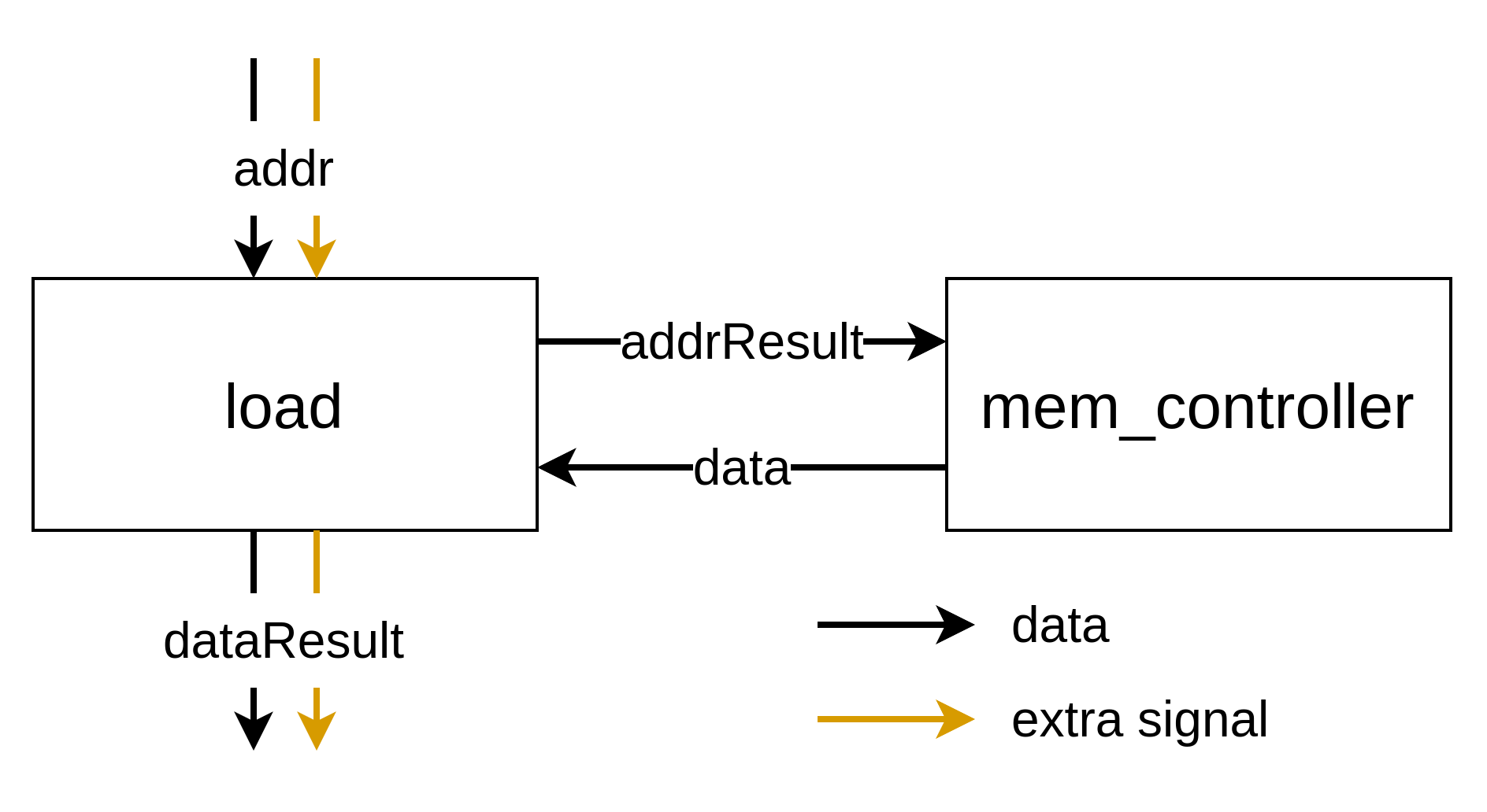
- The
addrResultanddataports, used to communicate with the memory controller, must be simple. - The
addranddataResultports must carry the same set of extra signals.
For the store operation, the structure is:
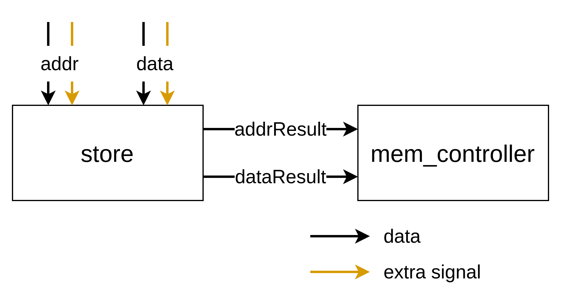
- The
addrResultanddataResultports, which interface with the memory controller, must also be simple. - The
addranddataports must have matching extra signals.
This design decision was discussed in the issue #214.
ConstantOp
While this operation falls under the default category, it’s worth highlighting due to the non-trivial way it handles control tokens with extra signals that trigger the emission of a constant value.
ConstantOp has one input (a ControlType to trigger the emission) and one output (a ChannelType). Like other operations, the extra signals of the input and output should match.
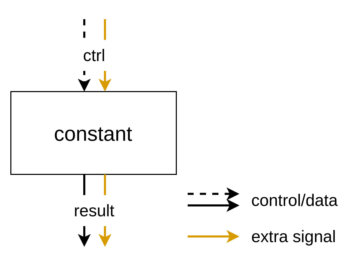
To ensure consistency for succeeding operations, ConstantOp must generate an output with extra signals. For example, if an adder expects a spec tag, the preceding ConstantOp must provide one.
However, since control tokens can now carry extra signals, a control token with extra signals may trigger ConstantOp (e.g., in some cases, a token from the basic block’s control network is used).
Therefore, we decided to forward the extra signals from the control input directly to the output token, rather than discarding them and hardcoding constant extra signal values in ConstantOp.
In other words, ConstantOp does not generate extra signals itself—this responsibility typically falls to a dedicated SourceOp, which supplies the control token for the succeeding ConstantOp. The values of these extra signals depend on the specific signals being propagated and are not discussed here.
This design decision was discussed in Issue #226 and a conversation in Pull Request #197.
2. Exploring the Implementation
Next, we’ll take a closer look at how these rules are implemented. We’ll begin by introducing some fundamental concepts.
Operations
Operations in the Handshake IR (such as MergeOp or ConstantOp) are defined declaratively in TableGen files (HandshakeOps.td or HandshakeArithOps.td).
Each operation has arguments, which are categorized into operands, attributes, and properties. We discuss only operands here. Operands represent the inputs to the RTL here. For example, ConditionalBranchOp has two operands: one for the condition and one for the data.
https://github.com/EPFL-LAP/dynamatic/blob/32df72b2255767c843ec4f251508b5a6179901b1/include/dynamatic/Dialect/Handshake/HandshakeOps.td#L457-L458
Some operands are variadic, meaning they can have a variable number of inputs. For example, the data operand of MuxOp is variadic.
https://github.com/EPFL-LAP/dynamatic/blob/32df72b2255767c843ec4f251508b5a6179901b1/include/dynamatic/Dialect/Handshake/HandshakeOps.td#L362-L363
More on operation arguments: https://mlir.llvm.org/docs/DefiningDialects/Operations/#operation-arguments
Each operation also has results, which represent the outputs of the RTL here. For instance, ConditionalBranchOp has two results, corresponding to the “true” and “false” branches.
https://github.com/EPFL-LAP/dynamatic/blob/32df72b2255767c843ec4f251508b5a6179901b1/include/dynamatic/Dialect/Handshake/HandshakeOps.td#L459-L460
Just like operands, some results are variadic (e.g., outputs of ForkOp).
More on operation results: https://mlir.llvm.org/docs/DefiningDialects/Operations/#operation-results
Types
You may notice that operands and results are often denoted by types like HandshakeType or ChannelType. In Handshake IR, types specify the kind of RTL port.
The base class of all types in the Handshake dialect is the HandshakeType class.
Most variables in the IR are either ChannelType or ControlType.
ChannelType– Represents a data port with data + valid + ready signals.ControlType– Represents a control port with valid + ready signals.
These types are defined in HandshakeTypes.td.
The actual operands have concrete instances of these types. For example, an operand of AddIOp (integer addition) has a ChannelType, meaning its actual type will be:
!handshake.channel<i32>(for 32-bit integers)!handshake.channel<i8>(for 8-bit integers)
Since ChannelType allows different data types, multiple type instances are possible.
Some HandshakeType instances may include extra signals beyond (data +) valid + ready. For example:
!handshake.channel<i32, [spec: i1]>!handshake.control<[spec: i1, tag: i8]>
Traits
Traits are constraints applied to operations. They serve various purposes, but here we discuss their use for type validation.
For example, In CompareOp, the lhs/rhs operands must have the same type instance (e.g., !handshake.channel<i32>). However, simply specifying ChannelType for each is not enough—without additional constraints, the operation could exist with mismatched types, like:
lhs: !handshake.channel<i8>rhs: !handshake.channel<i32>
To enforce type consistency, we apply the AllTypesMatch trait:
https://github.com/EPFL-LAP/dynamatic/blob/32df72b2255767c843ec4f251508b5a6179901b1/include/dynamatic/Dialect/Handshake/HandshakeArithOps.td#L67-L69
This ensures that both elements share the exact same type instance.
MLIR provides AllTypesMatch, but we’ve introduced similar traits:
AllDataTypesMatch– Ignores differences in extra signals.AllExtraSignalsMatch– Ensures the extra signals match, ignoring the data type (if exists).
Traits are sometimes called multi-entity constraints because they enforce relationships across multiple operands or results.
In contrast, types (or type constraints) are called single-entity constraints as they enforce properties on individual elements.
It’s worth noting that we sometimes use traits even in single-entity cases for consistency. For example, IsSimpleHandshake ensures the type doesn’t include any extra signals, while IsIntChannel ensures the channel’s data type is IntegerType.
More on constraints: https://mlir.llvm.org/docs/DefiningDialects/Operations/#constraints
Applying Traits to Operations
Now, let’s see how traits are applied to different operations to enforce extra signal consistency.
Operations Within a Basic Block
Most operations use the AllTypesMatch trait to ensure that extra signals remain consistent across all inputs and outputs. However, when operands and results have different data types—such as the condition (i1) and data input (variable type) in ConditionalBranchOp—the AllExtraSignalsMatch trait is applied instead.
MuxOp and CMergeOp
The following constraints ensure proper handling of extra signals:
MergingExtraSignals– Validates extra signal consistency across the data inputs and data output.AllDataTypesMatchWithVariadic– Ensures uniform data types across the data inputs and variadic data output.
Additionally, the selector port is of type SimpleChannel, as it does not carry extra signals.
MemPortOp (Load and Store)
The following constraints are enforced:
AllExtraSignalsMatch– Ensures extra signals match across corresponding ports.IsSimpleHandshake– Ensures that ports connected to the memory controller do not carry extra signals.AllDataTypesMatch– Maintains consistency betweenaddr/addrResultanddata/dataResultdata types.
More Information
The MLIR documentation can be complex, but it covers the key concepts well. You can check out the following links for more details:
https://mlir.llvm.org/docs/DefiningDialects/Operations
https://mlir.llvm.org/docs/DefiningDialects/AttributesAndTypes
Note
What Does “Same” Extra Signals Mean?
Comparing extra signals across handshake types is complex. In the IR, extra signals are written in a specific order, but essentially, the extra signals of a handshake type should be treated as a set, where the order doesn’t matter. For example, [spec: i1, tag: i8] and [tag: i8, spec: i1] should be handled identically. Currently, this comparison is not strictly enforced in the codebase, but this will be addressed in the future.
Upstream Extra Signals
At present, upstream extra signals are not well handled. For example, the constraints for MuxOp and CMergeOp do not seem to account for upstream cases. This needs to be updated in the future when the need arises.
Instantiation of MLIR Operations at C-Level
This document explains how to use placeholder functions in C to instantiate an MLIR operation within the Handshake dialect.
The following figure shows the current flow:
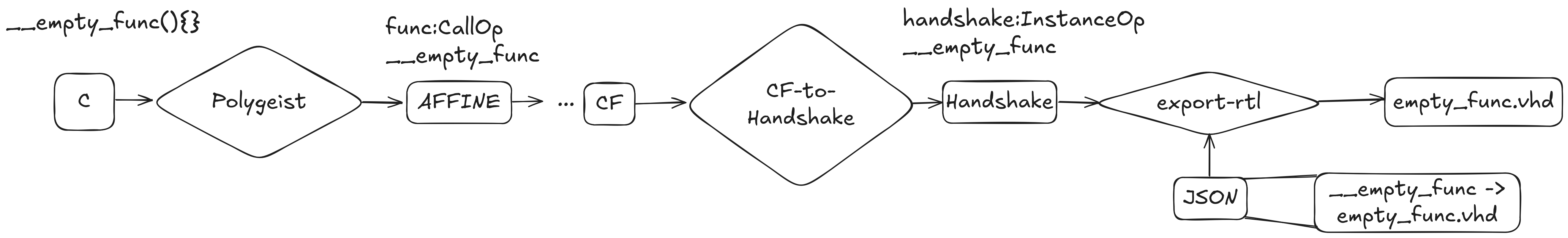
A placeholder function named in the format __name_component can be used to instantiate a specific MLIR operation at the C level. At the MLIR level, these functions are initially represented as an empty func:callOp. The callOp remains unchanged until the transformation pass from cf to handshake, where it is turned into a handshake:InstanceOp. These instances then continue through the processing flow.
The key step for this feature is the CfToHandshake lowering process. Dynamatic uses the callOp’s operands to determine inputs, outputs, and parameters of the handshake:InstanceOp. The following figure gives a quick overview of this process:

The rest of this document goes into details of this procedure.
1. Overview of Placeholder Functions
Placeholder functions can be declared at the C/C++ source level by using a double underscore __ prefix. These functions act as placeholders and should not have a definition, which ensures they are treated as external functions during lowering.
Argument variables are rewired inside of CfToHandshake based on their naming. In particular, arguments with the prefixes input_, output_, and parameter_ correspond to the inputs, outputs, and parameters of the InstanceOp.
Example:
void __new_component(int input_a, int output_b, int output_c, int parameter_bitw);
%output_c = __new_component %input_a, %output_b, {bitw = %paramter_bitw}
2. Variable Handling and Requirements
Variables passed as arguments to placeholder functions must follow these rules:
-
Naming Convention:
Inside the placeholder function definition, all arguments must have names that begin withinput_,output_, orparameter_. If there is any argument that does not follow any of these conventions, the code will throw an error. When defining the variables that will be passed into the placeholder function, any name can be chosen. For example://function definition using naming convention int __placeholder(int input_a, int output_b); int __init(); int main(){ .... //arbitrary names for variables int x; int y = __init(); __placeholder(x, y); .... }The MLIR operation
__placeholderwould receive as input x and as output y. -
Undefined Output Arguments:
Output arguments must be initialized using special__init*()functions. For example:void __placeholder(int input_a, int output_b); int __init1(); int main(){ .... // undefined output variable Var1 initialized using __init1() int Var1 = __init1(); __placeholder(.. , Var1); }Note that
__init1()follows the same style as placeholder functions (i.e., prefixed with__and left undefined), but is treated as a special case by the compiler. Each__init*function must return the correct type to match its associated output (e.g.,output_bis anint, so__init1()must returnint). If another output likeoutput_chas typefloat, you must define a new__init2()that returnsfloat.void __placeholder(int input_a, int output_b, float output_c); int __init1(); // used for int outputs float __init2(); // used for float outputsAll
__init*()functions must have unique names, but any name is valid as long as it starts with"__init". -
At Least One Output Required:
This is important since it’s expected that the return value of the MLIR op CallOp is replaced by a data result of InstanceOp. Therefore, InstanceOp should have at least one output. -
Inputs Must Not Be Initialized with
__init*():
These functions are exclusively used for outputs that are passed to placeholder functions. Inputs should be defined as usual and treated by the compiler in the standard way. If outputs variable are initialized with__init*()but are not an argument of the placeholder function, the produced IR will be invalid. Therefore, initialization via__init*()is permitted only for variables that are passed as output arguments to the placeholder, any other use is disallowed and triggers an assertion when exiting the pass. -
Parameters Must Be Constant:
Parameter arguments must be assigned constant values (e.g.,int bitw = 31;). This is necessary because parameters are converted into attributes on thehandshake.instance. If a parameter is not a constant, an assertion will fail during the conversion process. The following is a correct example://function definition using naming convention int __placeholder(int input_a, int output_b, int parameter_bitw); int __init(); int main(){ .... //arbitrary names for variables int x; int y = __init(); int z = 31; __placeholder(x, y, z); .... }In this case, the variable
zhas a constant value.
3. Important Assumptions
-
Correct usage of
__init*():__init*()functions should only initialize output arguments of the placeholder functions. If a variable defined by __init*() is not used by any placeholder, neither the variable nor its function definition is removed. This would leave an invalid IR, which is why we have an assertion in place that verifies this is not the case. -
At Least One Output:
Placeholder functions must include at least oneoutput_argument. -
Acyclic Data Dependencies:
There must be no cyclic data dependencies involving the outputs of placeholder functions used as inputs of the same placeholder function. This is due to limitations in the current rewiring logic. Cycles (e.g., output values used to compute their own input) could lead to invalid SSA or deadlock in the handshake IR. -
SSA domination: Each argument passed to the placeholder must be defined before its first use (i.e., it must dominate the call).
4. Additional Notes
-
Constants used to define parameters (e.g.,
bitw = 31) are not removed by the conversion pass. Instead, the users of those constants (i.e., placeholder call arguments) are removed. If the constants end up unused, they will be automatically cleaned up during the handshake canonicalization pass. -
For placeholder functions, the call’s return value is always replaced by the first result of the newly created
handshake.instance. We assume that placeholder functions always contain at least one output argument, which ensures that the first result is of a dataflow type. This is necessary to maintain consistency with the pre-transformation call, which also returned a dataflow value.
Why Parameter Constants Are Not Deleted Manually:
During the conversion, parameter values are extracted from arith.constant operations and embedded directly as attributes on the handshake.instance. These constants originate from the pre-transformation graph (i.e., before the function is rewritten).
Attempting to delete them inside of matchAndRewrite fails because MLIR’s conversion framework has already replaced or removed them with handshake constantOp. For example, you might hit errors like: “operation was already replaced”.
To avoid this, we do not erase the parameter constants manually. Any unused constants are cleaned up automatically by later passes, and importantly, they do not appear in the final handshake_export IR.
5. Pass Logic and matchAndRewrite Behavior
-
Functions named
__init*()are treated as legal and excluded from conversion. This allows them to remain temporarily in the IR until they’re explicitly removed later. -
All other placeholder functions (those using the
__placeholderpattern) entermatchAndRewrite.
Inside matchAndRewrite:

-
Functions are first differentiated from normal function calls. Non-placeholder calls are lowered using the standard logic (dashed arrows).
-
For placeholder functions, arguments are classified by naming convention by checking
handshake.arg_name:- Arguments starting with
input_are treated as inputs. output_arguments are used to construct result types and for the rewiring of the instance results.parameter_arguments must be constants and are converted to attributes on thehandshake:instanceOp.- If an argument does not follow the expected naming convention, an assertion will fail, informing the user that one of the arguments is incorrectly named.
- Additionally, after classification, the code verifies that the
output_list is not empty, since at least one output argument is required. If no outputs are found, a second assertion will fail.
- Arguments starting with
-
Mappings are built:
- For each output argument, the index is stored together with a list of users that consume that output inside a dictionary (
OutputConnections:indices → list of users). This dictionary will later be used for rewiring. - Similarly, for each parameter, we store its name and value in a dictionary (
parameterMap: names → constant values), for attribute conversion.
- For each output argument, the index is stored together with a list of users that consume that output inside a dictionary (
-
The placeholder function’s signature is rewritten to match the actual inputs and outputs post-conversion. This ensures the IR is valid and passes MLIR verification. If the function definition doesn’t correctly reflect the new instance format, MLIR verification fails and emits an error.
-
The
resultTypesare extracted from the rewritten function signature. After that, they are cast intoHandshakeResultTypes. TheOperandslist is cleaned up by removing outputs and parameters. Then, it consists of only inputs. -
A
handshake.instanceis created using theHandshakeResultTypesand cleanedOperandslist. -
Mappings are used to:
- Attach parameters as named attributes to the instance using
parameterMap. - Rewire all output users to use the corresponding instance results using
OutputConnections. The rewiring logic iterates over theInstanceOpOutputIndiceslist in order and replaces each output index with the corresponding result from the instance operation. This means that the position of each output index in the list determines which instance result it maps to. For example, if the output indices are(1, 3, 4, 7), then the rewiring will map them as follows:(1, 3, 4, 7) → (%4#0, %4#1, %4#2, %4#3)
- Attach parameters as named attributes to the instance using
6. Final Cleanup
-
Any
__init*()calls used to initialize output variables are removed during thematchAndRewriteconversion step, once their results have been replaced by the correspondinghandshake.instanceoutputs. -
After the full conversion is complete, if a
__init*()function definition has no remaining users, it is deleted as part of a post-pass cleanup step. If a__init*()function definition still has users an assertion will be triggered.
Important Note:
In case a variable was initialized using __init*() but wasn’t passed to placeholder function, that call @ __init*() will still be present in the IR and therefore will not allow for the deletion of __init*()’s function definition. This will cause an invalid IR. Hence why we assume correct usage of __init*() in 3. Important-Assumptions.
7. Data Dependency Assumption
This rewiring logic assumes that placeholder function calls are used in acyclic dataflow contexts. Specifically:
- No value returned by a placeholder is fed back (directly or indirectly) as an input to the same instance.
- All users of a placeholder output are dominated by its definition and reside in the same or nested blocks.
This assumption is important because rewiring outputs from an InstanceOp directly into operands that are evaluated before the instance could lead to cyclic data dependencies or violations of SSA dominance in the IR.
Currently, loop-carried dependencies (e.g., in
for/whileloops) are not handled explicitly. This logic must be revisited if support for loop-aware rewrites or control-flow merges is added.
8. Example
Consider the Example below, where we use a placeholder function that produces two outputs that are then used for simple operations:
Example Code
//placeholder with two outputs
void __placeholder(int input_a, int output_b, int output_c, int parameter_BITWIDTH);
int __init1();

int hw_inst() {
  int bitw = 31;
  int a = 11;
  int b = __init1();
  int c = __init1();
  __placeholder(a, b, c, bitw);
  // using inputs and outputs for computation
  int result = a - b + c;
  return result;
}
Next, take a look at the pre- and post-transformation IR. We see that the calls to @__init*() disappear, the instance now correctly reflects the expected behaviour, and all outputs have been rewired. Additionally, the parameter becomes an attribute of the newly created instance.
Pre-Transformation IR
module {
  func.func @hw_inst() -> i32 {
    %c31_i32 = arith.constant {handshake.name = "constant0"} 31 : i32
    %c11_i32 = arith.constant {handshake.name = "constant1"} 11 : i32
    %0 = call @__init1() {handshake.name = "call0"} : () -> i32
    %1 = call @__init1() {handshake.name = "call1"} : () -> i32
    call @__placeholder(%c11_i32, %0, %1, %c31_i32) {handshake.name = "call2"} : (i32, i32, i32, i32) -> ()
    %2 = arith.subi %c11_i32, %0 {handshake.name = "subi0"} : i32
    %3 = arith.addi %2, %1 {handshake.name = "addi0"} : i32
    return {handshake.name = "return0"} %3 : i32
  }
  func.func private @__init1() -> i32
  func.func private @__placeholder(i32 {handshake.arg_name = "input_a"}, i32 {handshake.arg_name = "output_b"}, i32 {handshake.arg_name = "output_c"}, i32 {handshake.arg_name = "parameter_BITWIDTH"})
}
Notice that %0 and %1 are the output variables. They are initialized using __init1(), passed to the __placeholder() call, and later used in the computation.
Post-Transformation IR
module {
  handshake.func @hw_inst(%arg0: !handshake.control<>, ...) -> (!handshake.channel<i32>, !handshake.control<>) attributes {argNames = ["start"], resNames = ["out0", "end"]} {
    %0 = source {handshake.bb = 0 : ui32, handshake.name = "source0"} : <>
    %1 = constant %0 {handshake.bb = 0 : ui32, handshake.name = "constant0", value = 31 : i32} : <>, <i32>
    %2 = source {handshake.bb = 0 : ui32, handshake.name = "source1"} : <>
    %3 = constant %2 {handshake.bb = 0 : ui32, handshake.name = "constant1", value = 11 : i32} : <>, <i32>
    %4:3 = instance @__placeholder(%3, %arg0) {BITWIDTH = 31 : i32, handshake.bb = 0 : ui32, handshake.name = "call2"} : (!handshake.channel<i32>, !handshake.control<>) -> (!handshake.channel<i32>, !handshake.channel<i32>, !handshake.control<>)
    %5 = subi %3, %4#0 {handshake.bb = 0 : ui32, handshake.name = "subi0"} : <i32>
    %6 = addi %5, %4#1 {handshake.bb = 0 : ui32, handshake.name = "addi0"} : <i32>
    end {handshake.bb = 0 : ui32, handshake.name = "end0"} %6, %arg0 : <i32>, <>
  }
  handshake.func private @__placeholder(!handshake.channel<i32>, !handshake.control<>, ...) -> (!handshake.channel<i32>, !handshake.channel<i32>, !handshake.control<>) attributes {argNames = ["input_a", "start"], resNames = ["out0", "out1", "end"]}
}
The @__placeholder instance now produces three results: two data outputs (%4#0, %4#1) and one control signal. The computation that previously used %0 and %1 has been rewired to use these instance results. All __init1() calls and their function signature have been removed from the IR.
Note: The constant value used for the parameter (
BITWIDTH = 31) remains in the IR for now but will be eliminated during the final export pass, as it is embedded into the instance as an attribute.
9. Testing
A FileCheck test is available to validate the correctness of the transformation. It can be found in test/Transforms/handshake-hw-inst.mlir and it verifies the correct creation of multi-output handshake::InstanceOps, rewiring of outputs, and conversion of parameters into attributes.
10. Related References
This implementation and design were informed by discussions and iterations captured in the following GitHub entries:
-
Issue #321: Incomplete Generation of MLIR OP at C-Level
Documents early investigation into missing MLIR operations for multi-output functions. -
PR #384: Add Argument Classification Based on Naming Convention in CfToHandshake
Introduces the initial support for placeholder function classification and output rewiring. -
PR #467: Complete Support for Multi-Output MLIR Operations
Refines the lowering logic, finalizes__init*()and parameter handling, and forms the basis of this documentation.
An MLIR Primer
This tutorial will introduce you to MLIR and its core constructs. It is intended as a short and very incomplete yet pragmatic first look into the framework for newcomers, and will provide you with valuable “day-0” information that you’re likely to need as soon as you start developing in Dynamatic. At many points, this tutorial will reference the official and definitely more complete MLIR documentation, which you are invited to look up whenever you require more in-depth information about a particular concept. While this document is useful to get an initial idea of how MLIR works and of how to manipulate its data-structures, we strongly recommend the reader to follow a “learn by doing” philosophy. Reading documentation, especially of complex frameworks like MLIR, will only get you so far. Practice is the path toward actual understanding and mastering in the long run.
Table of contents
- High-level structure | What are the core data-structures used throughout MLIR?
- Traversing the IR | How does one traverse the recursive IR top-to-bottom and bottom-to-top?
- Values | What are values and how are they used by operations?
- Operations | What are operations and how does one manipulate them?
- Regions | What are regions and what kind of abstraction can they map to?
- Blocks | What are blocks and block arguments?
- Attributes | What are attributes and what are they used for?
- Dialects | What are MLIR dialects?
- Printing to the console | What are the various ways of printing to the console?
High-level structure
From the language reference:
MLIR is fundamentally based on a graph-like data structure of nodes, called
Operations, and edges, calledValues. EachValueis the result of exactly oneOperationorBlockArgument, and has aValueTypedefined by the type system. Operations are contained inBlocks andBlocks are contained inRegions.Operations are also ordered within their containing block andBlocks are ordered in their containing region, although this order may or may not be semantically meaningful in a given kind of region). Operations may also contain regions, enabling hierarchical structures to be represented.
All of these data-structures can be manipulated in C++ using their respective types (which are typesetted in the above paragraph). In addition, they can all be printed to a text file (by convention, a file with the .mlir extension) and parsed back to their in-memory representation at any point.
To summarize, every MLIR file (*.mlir) is recursively nested. It starts with a top-level operation (often, an mlir::ModuleOp) which may contain nested regions, each of which may contain an ordered list of nested blocks, each of which may contain an ordered list of nested operations, after which the hierarchy repeats.
Traversing the IR
From top to bottom
Thanks to MLIR’s recursively nested structure, it is very easy to traverse the entire IR recursively. Consider the following C++ function which finds and recursively traverses all operations nested within a provided operation.
void traverseIRFromOperation(mlir::Operation *op) {
for (mlir::Region ®ion : op->getRegions()) {
for (mlir::Block &block : region.getBlocks()) {
for (mlir::Operation &nestedOp : block.getOperations()) {
llvm::outs() << "Traversing operation " << op << "\n";
traverseIRFromOperation(&nestedOp);
}
}
}
}
MLIR also exposes the walk method on the Operation, Region, and block types. walk takes as single argument a callback method that will be invoked recursively for all operations recursively nested under the receiving entity.
// Let block be a Block&
mlir::Block &block = ...;

// Walk all operations nested in the block
block.walk([&](mlir::Operation *op) {
  llvm::outs() << "Traversing operation " << op << "\n";
});
From bottom to top
One may also get the parent entities of a given operation/region/block.
// Let op be an Operation*
mlir::Operation* op = ...;

// All of the following functions may return a nullptr in case the receiving
// entity is currently unattached to a parent block/region/op or is a top-level
// operation

// Get the parent block the operation immediately belongs to
mlir::Block *parentBlock = op->getBlock();
// Get the parent region the operation immediately belongs to
mlir::Region *parentRegion = op->getParentRegion();
// Get the parent operation the operation immediately belongs to
mlir::Operation *parentOp = op->getParentOp();

// Get the parent region the block immediately belongs to
mlir::Region *blockParentRegion = parentBlock->getParent();
assert(parentRegion == blockParentRegion);
// Get the parent operation the block immediately belongs to
mlir::Operation *blockParentOp = parentBlock->getParentOp();
assert(parentOp == blockParentOp);

// Get the parent operation the region immediately belongs to
mlir::Operation *regionParentOp = parentRegion->getParentOp();
assert(parentOp == regionParentOp);
Values
Values are the edges of the graph-like structure that MLIR models. Their corresponding C++ type is mlir::Value. All values are typed using either a built-in type or a custom user-defined type (the type of a value is itself a C++ type called Type), which may change at runtime but is subject to verification constraints imposed by the context in which the value is used. Values are either produced by operations as operation results (mlir::OpResult, which is a subtype of mlir::Value) or are defined by blocks as part of their block arguments (mlir::BlockArgument, also a subtype of mlir::Value). They are consumed by operations as operation operands. A value may have 0 or more uses, but should have exactly one producer (an operation or a block).
The following C++ snippet shows how to identify the type and producer of a value and prints the index of the producer’s operation result/block argument that the value corresponds to.
// Let value be a Value
mlir::Value value = ...;

// Get the value's type and check whether it is an integer type
mlir::Type valueType = value.getType();
if (mlir::isa<mlir::IntegerType>(valueType))
  llvm::outs() << "Value has an integer type\n";
else
  llvm::outs() << "Value does not have an integer type\n";

// Get the value's producer (either a block, if getDefiningOp returns a nullptr,
// or an operation)
if (mlir::Operation *definingOp = value.getDefiningOp()) {
  // Value is a result of its defining operation and can safely be casted as such
  mlir::OpResult valueRes = cast<mlir::OpResult>(value);
  // Find the index of the defining operation result that corresponds to the value
  llvm::outs() << "Value is result number" << valueRes.getResultNumber(); << "\n";
} else {
  // Value is a block argument and can safely be casted as such
  mlir::BlockArgument valueArg = cast<mlir::BlockArgument>(value);
  // Find the index of the block argument that corresponds to the value
  llvm::outs() << "Value is result number" << valueArg.getArgNumber() << "\n";
}
The following C++ snippet shows how to iterate through all the operations that use a particular value as operand. Note that the number of uses may be equal or larger than the number of users because a single user may use the same value multiple times (but at least once) in its operands.
// Let value be a Value
mlir::Value value = ...;

// Iterate over all uses of the value (i.e., over operation operands that equal
// the value)
for (mlir::OpOperand &use : value.getUses()) {
  // Get the owner of this particular use
  mlir::Operation *useOwner = use.getOwner();
  llvm::outs() << "Value is used as operand number "
               << use.getOperandNumber() << " of operation "
               << useOwner << "\n";
}

// Iterate over all users of the value
for (mlir::Operation *user : value.getUsers())
  llvm::outs() << "Value is used as an operand of operation " << user << "\n";
Operations
In MLIR, everything is about operations. Operations are like “opaque functions” to MLIR; they may represent some abstraction (e.g., a function, with a mlir::func::FuncOp operation) or perform some computation (e.g., an integer addition, with a mlir::arith::AddIOp). There is no fixed set of operations; users may define their own operations with custom semantics and use them at the same time as MLIR-defined operations. Operations:
- are identified by a unique string
- can take 0 or more operands
- can return 0 or more results
- can have attributes (i.e., constant data stored in a dictionary)
The C++ snippet below shows how to get an operation’s information from C++.
// Let op be an Operation*
mlir::Operation* op = ...;

// Get the unique string identifying the type of operation
mlir::StringRef name = op->getName().getStringRef();

// Get all operands of the operation
mlir::OperandRange allOperands = op->getOperands();
// Get the number of operands of the operation
size_t numOperands = op->getNumOperands();
// Get the first operand of the operation (will fail if 0 >= op->getNumOperands())
mlir::Value firstOperand = op->getOperand(0);

// Get all results of the operation
mlir::ResultRange allResults = op->getResults();
// Get the number of results of the operation
size_t numResults = op->getNumResults();
// Get the first result of the operation (will fail if 0 >= op->getNumResults())
mlir::OpResult firstResult = op->getResult(0);

// Get all attributes of the operation
mlir::DictionaryAttr allAttributes = op->getAttrDictionary();

// Try to get an attribute of the operation with name "attr-name"
mlir::Attribute someAttr = op->getAttr("attr-name");
if (someAttr)
  llvm::outs() << "Attribute attr-name exists\n";
else
  llvm::outs() << "Attribute attr-name does not exist\n";

// Try to get an integer attribute of the operation with name "attr-name"
mlir::IntegerAttr someIntAttr = op->getAttrOfType<IntegerAttr>("attr-name");
if (someAttr)
  llvm::outs() << "Integer attribute attr-name exists\n";
else
  llvm::outs() << "Integer attribute attr-name does not exist\n";
Op vs Operation
As we saw above, you can manipulate any operation in MLIR using the “opaque” Operation type (usually, you do so through an Operation*) which provides a generic API into an operation instance. However, there exists another type, Op, whose derived classes model a specific type of operation (e.g., an integer addition with a mlir::arith::AddIOp). From the official documentation:
Opderived classes act as smart pointer wrapper around aOperation*, provide operation-specific accessor methods, and type-safe properties of operations. (…) A side effect of this design is that we always pass aroundOpderived classes “by-value”, instead of by reference or pointer.
Whenever you want to manipulate an operation of a specific type, you should do so through its actual type that derives from Op. Fortunately, it is easy to identify the actual type of an Operation* using MLIR’s casting infrastructure. The following snippet shows a few different methods to check whether an opaque Operation* is actually an integer addition (mlir::arith::AddIOp).
// Let op be an Operation*
mlir::Operation* op = ...;

// Method 1: isa followed by cast
if (mlir::isa<mlir::arith::AddIOp>(op)) {
  // We now op is actually an integer addition, so we can safely cast it
  // (mlir::cast fails if the operation is not of the indicated type)
  mlir::arith::AddIOp addOp = mlir::cast<mlir::arith::AddIOp>(op);
  llvm::outs() << "op is an integer addition!\n";
}

// Method 2: dyn_cast followed by nullptr check
// dyn_cast returns a valid pointer if the operation is of the indicated type
// and returns nullptr otherwise
mlir::arith::AddIOp addOp = mlir::dyn_cast<mlir::arith::AddIOp>(op)
if (addOp) {
  llvm::outs() << "op is an integer addition!\n";
}

// Method 3: simultaneous dyn_cast and nullptr check
// Using the following syntax, we can simultaneously assign addOp and check if
// it is a nullptr
if (mlir::arith::AddIOp addOp = mlir::dyn_cast<mlir::arith::AddIOp>(op)) {
  llvm::outs() << "op is an integer addition!\n";
}
Once you have a specific derived class of Op on hand, you can access methods that are specific to the operation type in question. For example, for all operation operands, MLIR will automatically generate an accessor method with the name get<operand name in CamelCase>. For example, mlir::arith::AddIOp has two operands named lhs and rhs that represent, respectively, the left-hand-side and right-hand-side of the addition. It is possible to get these operands using their name instead of their index with the following code.
// Let addOp be an integer Operation
mlir::arith::AddIOp addOp = ...;

// Get first operand (lhs)
mlir::Value firstOperand = addOp->getOperand(0);
mlir::Value lhs = addO.getLhs();
assert(firstOperand == lhs);

// Get second operand (rhs)
mlir::Value secondOperand = addOp->getOperand(1);
mlir::Value rhs = addO.getRhs();
assert(secondOperand == rhs);
When iterating over the operations inside a region or block, it’s possible to only iterate over operations of a specific type using the getOps<OpTy> method.
// Let region be a Region&
mlir::Region ®ion = ...;
// Iterate over all integer additions inside the region's blocks
for (mlir::arith::AddIOp addOp : region.getOps<mlir::arith::AddIOp>())
llvm::outs() << "Found an integer operation!\n";
// Equivalently, we can first iterate over blocks, then operations
for (Block &block : region.getBlocks())
for (mlir::arith::AddIOp addOp : block.getOps<mlir::arith::AddIOp>())
llvm::outs() << "Found an integer operation!\n";
// Equivalently, without using getOps<OpTy>
for (Block &block : region.getBlocks())
for (Operation* op : block.getOperations())
if (mlir::arith::AddIOp addOp = mlir::dyn_cast<mlir::arith::AddIOp>(op))
llvm::outs() << "Found an integer operation!\n";
The walk method similarly allows one to specify a type of operation to recursively iterate on inside the callback’s signature.
// Let block be a Block&
mlir::Block &block = ...;

// Walk all integer additions nested in the block
block.walk([&](mlir::arith::AddIOp op) {
  llvm::outs() << "Found an integer operation!\n";
});

// Equivalently, without using the operation type in the callback's signature
block.walk([&](Operation *op) {
  if (mlir::isa<mlir::arith::AddIOp>(op))
    llvm::outs() << "Found an integer operation!\n";
});
Regions
From the language reference:
A region is an ordered list of MLIR blocks. The semantics within a region is not imposed by the IR. Instead, the containing operation defines the semantics of the regions it contains. MLIR currently defines two kinds of regions: SSACFG regions, which describe control flow between blocks, and Graph regions, which do not require control flow between blocks.
The first block in a region, called the entry block, is special; its arguments also serve as the region’s arguments. The source of these arguments is defined by the semantics of the parent operation. When control flow enters a region, it always begins in the entry block. Regions may also produce a list of values when control flow leaves the region. Again, the parent operation defines the relation between the region results and its own results. All values defined within a region are not visible from outside the region (they are encapsulated). However, by default, a region can reference values defined outside of itself if these values would have been usable by the region’s parent operation operands.
A function body (i.e., the region inside a mlir::func::FuncOp operation) is an example of an SSACFG region, where each block represents a control-free sequence of operations that executes sequentially. The last operation of each block, called the terminator operation (see the next sextion), identifies where control flow goes next; either to another block, called a successor block in this context, inside the function body (in the case of a branch-like operation) or back to the parent operation (in the case of a return-like operation).
Graph regions, on the other hand, can only contain a single basic block and are appropriate to represent concurrent semantics without control flow. This makes them the perfect representation for dataflow circuits which have no notion of sequential execution. In particular (from the language reference)
All values defined in the graph region as results of operations are in scope within the region and can be accessed by any other operation in the region. In graph regions, the order of operations within a block and the order of blocks in a region is not semantically meaningful and non-terminator operations may be freely reordered.
Blocks
A block is an ordered list of MLIR operations. The last operation in a block must be a terminator operation, unless it is the single block of a region whose parent operation has the NoTerminator trait (mlir::ModuleOp is such an operation).
As mentioned in the prior section on MLIR values, blocks may have block arguments. From the language reference:
Blocks in MLIR take a list of block arguments, notated in a function-like way. Block arguments are bound to values specified by the semantics of individual operations. Block arguments of the entry block of a region are also arguments to the region and the values bound to these arguments are determined by the semantics of the parent operation. Block arguments of other blocks are determined by the semantics of terminator operations (e.g., branch-like operations) which have the block as a successor.
In SSACFG regions, these block arguments often implicitly represent the passage of control-flow dependent values. They remove the need for PHI nodes that many other SSA IRs employ (like LLVM IR).
Attributes
For this section, you are simply invited to read the relevant part of the language reference, which is very short.
In summary, attributes are used to attach data/information to operations that cannot be expressed using a value operand. Additionally, attributes allow us to propagate meta-information about operations down the lowering pipeline. This is useful whenever, for example, some analysis can only be performed at a “high IR level” but its results only become relevant at a “low IR level”. In these situations, the analysis’s results would be attached to relevant operations using attributes, and these attributes would then be propagated through lowering passes until the IR reaches the level where the information must be acted upon.
Dialects
For this section, you are also simply invited to read the relevant part of the language reference, which is very short.
The Handshake dialect, defined in the dynamatic::handshake namespace, is core to Dynamatic. Handshake allows us to represent dataflow circuits inside graph regions. Throughout the repository, whenever we mention “Handshake-level IR”, we are referring to an IR that contains Handshake operations (i.e., dataflow components), which together make up a dataflow circuit.
Printing to the console
Printing to stdout and stderr
LLVM/MLIR has wrappers around the standard program output streams that you should use whenever you would like something displayed on the console. These are llvm::outs() (for stdout) and llvm::errs() (for stderr), see their usage below.
// Let op be an Operation*
Operation *op = ...;

// Print to standard output (stdout)
llvm::outs() << "This will be printed on stdout!\n";

// Print to standard error (stderr)
llvm::errs() << "This will be printed on stderr!\n"
             << "As with std::cout and std::cerr, entities to print can be "
             << "piped using the '<<' C++ operator as long as they are "
             << "convertible to std::string, like the integer " << 10
             << " or an MLIR operation " << op << "\n";
caution
Dynamatic’s optimizer prints the IR resulting from running all the passes it was asked to run to standard output. As a consequence you should never explicitly print anything to stdout yourself, as it will mix up with the IR text serialization. Instead, all error messages should go to stderr.
Printing information related to an operation
You will regularly want to print a message to stdout/stderr and attach it to a specific operation that it relates to. While you could just use llvm::outs() or llvm::errs() and pipe the operation in question after the message (as shown above), MLIR has very convenient methods that allow you to achieve the same task more elegantly in code and with automatic output formatting; the operation instance will be (pretty-)printed with your custom message next to it.
// Let op be an Operation*
Operation *op = ...;

// Report an error on the operation
op->emitError() << "My error message";
// Report a warning on the operation
op->emitWarning() << "My warning message";
// Report a remark on the operation
op->emitRemark() << "My remark message";
Signal Manager
The signal manager wraps each unit (e.g., addi, buffer, etc.) and forwards extra signals.
Signal managers are implemented within the framework of the Python-based, generation-oriented beta backend for VHDL. The implementation files can be found under experimental/tools/unit-generators/vhdl/generators/support/signal_manager. Custom signal managers specific to individual units can also be implemented in their respective unit files.
Design Principles
When existing signal managers don’t fit your needs, we encourage you to create a new one using small, concrete helper functions. These functions are designed to work like Lego bricks, allowing you to easily assemble a custom signal manager tailored to your case.
Rather than extending the few existing signal managers, we recommend somewhat reinventing new ones. Extending the current signal managers can lead to highly parameterized, monolithic designs that are difficult to modify and understand. In contrast, this approach promotes modularity and simplicity, improving clarity and maintainability. While reinventing may seem repetitive, the small helper functions can take care of the tedious parts, keeping the implementation concrete and manageable.
Handling Different Extra Signals
The following illustration (by @murphe67) shows how the muli signal manager handles both spec and tag. The forwarding behavior differs between them: spec ORs two signals, while tag selects one and discards the other.
Although you can introduce as many signal managers as needed, since they all use common helper functions, you can define the forwarding semantics in a single place (generate_forwarding_expression_for_signal in signal_manager/utils/forwarding.py). This ensures consistency and reuse across all instances.
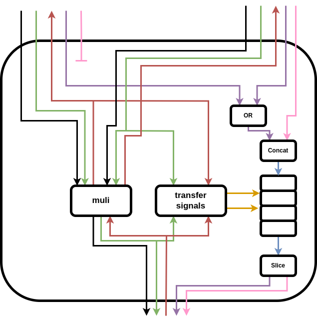
Examples
Below are some examples of signal managers. These can serve as references for understanding signal managers or for creating your own.
cond_br
The cond_br unit uses the default signal manager, which is provided in signal_manager/default.py.
library ieee;
use ieee.std_logic_1164.all;
use ieee.numeric_std.all;
use work.types.all;

-- Entity of signal manager
entity handshake_cond_br_2 is
  port(
    clk : in std_logic;
    rst : in std_logic;
    data : in std_logic_vector(32 - 1 downto 0);
    data_valid : in std_logic;
    data_ready : out std_logic;
    data_spec : in std_logic_vector(1 - 1 downto 0);
    condition : in std_logic_vector(1 - 1 downto 0);
    condition_valid : in std_logic;
    condition_ready : out std_logic;
    condition_spec : in std_logic_vector(1 - 1 downto 0);
    trueOut : out std_logic_vector(32 - 1 downto 0);
    trueOut_valid : out std_logic;
    trueOut_ready : in std_logic;
    trueOut_spec : out std_logic_vector(1 - 1 downto 0);
    falseOut : out std_logic_vector(32 - 1 downto 0);
    falseOut_valid : out std_logic;
    falseOut_ready : in std_logic;
    falseOut_spec : out std_logic_vector(1 - 1 downto 0)
  );
end entity;

-- Architecture of signal manager (normal)
architecture arch of handshake_cond_br_2 is
begin
  -- Forward extra signals to output ports
  trueOut_spec <= data_spec or condition_spec;
  falseOut_spec <= data_spec or condition_spec;

  inner : entity work.handshake_cond_br_2_inner(arch)
    port map(
      clk => clk,
      rst => rst,
      data => data,
      data_valid => data_valid,
      data_ready => data_ready,
      condition => condition,
      condition_valid => condition_valid,
      condition_ready => condition_ready,
      trueOut => trueOut,
      trueOut_valid => trueOut_valid,
      trueOut_ready => trueOut_ready,
      falseOut => falseOut,
      falseOut_valid => falseOut_valid,
      falseOut_ready => falseOut_ready
    );
end architecture;
muli
The muli unit uses the buffered signal manager, located in signal_manager/buffered.py. While it maintains the default signal forwarding, like the default signal manager, it also handles data path latency by introducing an internal FIFO.
library ieee;
use ieee.std_logic_1164.all;
use ieee.numeric_std.all;
use work.types.all;

-- Entity of signal manager
entity handshake_muli_0 is
  port(
    clk : in std_logic;
    rst : in std_logic;
    lhs : in std_logic_vector(32 - 1 downto 0);
    lhs_valid : in std_logic;
    lhs_ready : out std_logic;
    lhs_spec : in std_logic_vector(1 - 1 downto 0);
    rhs : in std_logic_vector(32 - 1 downto 0);
    rhs_valid : in std_logic;
    rhs_ready : out std_logic;
    rhs_spec : in std_logic_vector(1 - 1 downto 0);
    result : out std_logic_vector(32 - 1 downto 0);
    result_valid : out std_logic;
    result_ready : in std_logic;
    result_spec : out std_logic_vector(1 - 1 downto 0)
  );
end entity;

-- Architecture of signal manager (buffered)
architecture arch of handshake_muli_0 is
  signal buff_in, buff_out : std_logic_vector(1 - 1 downto 0);
  signal transfer_in, transfer_out : std_logic;
begin
  -- Transfer signal assignments
  transfer_in <= lhs_valid and lhs_ready;
  transfer_out <= result_valid and result_ready;

  -- Concat/split extra signals for buffer input/output
  buff_in(0 downto 0) <= lhs_spec or rhs_spec;
  result_spec <= buff_out(0 downto 0);

  inner : entity work.handshake_muli_0_inner(arch)
    port map(
      clk => clk,
      rst => rst,
      lhs => lhs,
      lhs_valid => lhs_valid,
      lhs_ready => lhs_ready,
      rhs => rhs,
      rhs_valid => rhs_valid,
      rhs_ready => rhs_ready,
      result => result,
      result_valid => result_valid,
      result_ready => result_ready
    );

  -- Generate ofifo to store extra signals
  -- num_slots = 4, bitwidth = 1
  buff : entity work.handshake_muli_0_buff(arch)
    port map(
      clk => clk,
      rst => rst,
      ins => buff_in,
      ins_valid => transfer_in,
      ins_ready => open,
      outs => buff_out,
      outs_valid => open,
      outs_ready => transfer_out
    );
end architecture;
The illustration of this circuit (by @murphe67) looks like this:
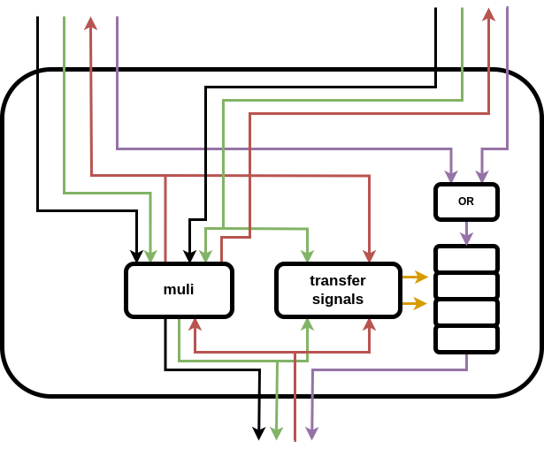
merge
The merge unit uses the concat signal manager, found in signal_manager/concat.py, to concatenate extra signals with the data signal. This behavior is not possible with the default signal forwarding.
library ieee;
use ieee.std_logic_1164.all;
use ieee.numeric_std.all;
use work.types.all;

-- Entity of signal manager
entity merge_0 is
  port(
    clk : in std_logic;
    rst : in std_logic;
    ins : in data_array(2 - 1 downto 0)(32 - 1 downto 0);
    ins_valid : in std_logic_vector(2 - 1 downto 0);
    ins_ready : out std_logic_vector(2 - 1 downto 0);
    ins_0_spec : in std_logic_vector(1 - 1 downto 0);
    ins_0_tag0 : in std_logic_vector(8 - 1 downto 0);
    ins_1_spec : in std_logic_vector(1 - 1 downto 0);
    ins_1_tag0 : in std_logic_vector(8 - 1 downto 0);
    outs : out std_logic_vector(32 - 1 downto 0);
    outs_valid : out std_logic;
    outs_ready : in std_logic;
    outs_spec : out std_logic_vector(1 - 1 downto 0);
    outs_tag0 : out std_logic_vector(8 - 1 downto 0)
  );
end entity;

-- Architecture of signal manager (concat)
architecture arch of merge_0 is
  signal ins_concat : data_array(1 downto 0)(40 downto 0);
  signal ins_concat_valid : std_logic_vector(1 downto 0);
  signal ins_concat_ready : std_logic_vector(1 downto 0);
  signal outs_concat : std_logic_vector(40 downto 0);
  signal outs_concat_valid : std_logic;
  signal outs_concat_ready : std_logic;
begin
  -- Concate/slice data and extra signals
  ins_concat(0)(32 - 1 downto 0) <= ins(0);
  ins_concat(0)(32 downto 32) <= ins_0_spec;
  ins_concat(0)(40 downto 33) <= ins_0_tag0;
  ins_concat(1)(32 - 1 downto 0) <= ins(1);
  ins_concat(1)(32 downto 32) <= ins_1_spec;
  ins_concat(1)(40 downto 33) <= ins_1_tag0;
  ins_concat_valid <= ins_valid;
  ins_ready <= ins_concat_ready;
  outs <= outs_concat(32 - 1 downto 0);
  outs_spec <= outs_concat(32 downto 32);
  outs_tag0 <= outs_concat(40 downto 33);
  outs_valid <= outs_concat_valid;
  outs_concat_ready <= outs_ready;

  inner : entity work.merge_0_inner(arch)
    port map(
      clk => clk,
      rst => rst,
      ins => ins_concat,
      ins_valid => ins_concat_valid,
      ins_ready => ins_concat_ready,
      outs => outs_concat,
      outs_valid => outs_concat_valid,
      outs_ready => outs_concat_ready
    );
end architecture;
select (custom signal manager)
library ieee;
use ieee.std_logic_1164.all;
use ieee.numeric_std.all;
use work.types.all;

-- Entity of signal manager
entity select_0 is
  port(
    clk : in std_logic;
    rst : in std_logic;
    condition : in std_logic_vector(1 - 1 downto 0);
    condition_valid : in std_logic;
    condition_ready : out std_logic;
    condition_spec : in std_logic_vector(1 - 1 downto 0);
    trueValue : in std_logic_vector(32 - 1 downto 0);
    trueValue_valid : in std_logic;
    trueValue_ready : out std_logic;
    trueValue_spec : in std_logic_vector(1 - 1 downto 0);
    falseValue : in std_logic_vector(32 - 1 downto 0);
    falseValue_valid : in std_logic;
    falseValue_ready : out std_logic;
    falseValue_spec : in std_logic_vector(1 - 1 downto 0);
    result : out std_logic_vector(32 - 1 downto 0);
    result_valid : out std_logic;
    result_ready : in std_logic;
    result_spec : out std_logic_vector(1 - 1 downto 0)
  );
end entity;

-- Architecture of selector signal manager
architecture arch of select_0 is
  signal trueValue_inner : std_logic_vector(32 downto 0);
  signal trueValue_inner_valid : std_logic;
  signal trueValue_inner_ready : std_logic;
  signal falseValue_inner : std_logic_vector(32 downto 0);
  signal falseValue_inner_valid : std_logic;
  signal falseValue_inner_ready : std_logic;
  signal result_inner_concat : std_logic_vector(32 downto 0);
  signal result_inner_concat_valid : std_logic;
  signal result_inner_concat_ready : std_logic;
  signal result_inner : std_logic_vector(31 downto 0);
  signal result_inner_valid : std_logic;
  signal result_inner_ready : std_logic;
  signal result_inner_spec : std_logic_vector(0 downto 0);
begin
  -- Concatenate extra signals
  trueValue_inner(32 - 1 downto 0) <= trueValue;
  trueValue_inner(32 downto 32) <= trueValue_spec;
  trueValue_inner_valid <= trueValue_valid;
  trueValue_ready <= trueValue_inner_ready;
  falseValue_inner(32 - 1 downto 0) <= falseValue;
  falseValue_inner(32 downto 32) <= falseValue_spec;
  falseValue_inner_valid <= falseValue_valid;
  falseValue_ready <= falseValue_inner_ready;
  result_inner <= result_inner_concat(32 - 1 downto 0);
  result_inner_spec <= result_inner_concat(32 downto 32);
  result_inner_valid <= result_inner_concat_valid;
  result_inner_concat_ready <= result_inner_ready;

  -- Forwarding logic
  result_spec <= condition_spec or result_inner_spec;

  result <= result_inner;
  result_valid <= result_inner_valid;
  result_inner_ready <= result_ready;

  inner : entity work.select_0_inner(arch)
    port map(
      clk => clk,
      rst => rst,
      condition => condition,
      condition_valid => condition_valid,
      condition_ready => condition_ready,
      trueValue => trueValue_inner,
      trueValue_valid => trueValue_inner_valid,
      trueValue_ready => trueValue_inner_ready,
      falseValue => falseValue_inner,
      falseValue_valid => falseValue_inner_valid,
      falseValue_ready => falseValue_inner_ready,
      result => result_inner_concat,
      result_ready => result_inner_concat_ready,
      result_valid => result_inner_concat_valid
    );
end architecture;
spec_commit
The spec_save_commit unit is used for speculation. It uses the spec_units signal manager, located in signal_manager/spec_units.py.
When spec_save_commit handles both spec: i1 and tag0: i8, it concatenates tag0 to the data while propagating spec to the inner unit. Additionally, it doesn’t concatenate the control signal, as it doesn’t carry any extra signals.
library ieee;
use ieee.std_logic_1164.all;
use ieee.numeric_std.all;
use work.types.all;

-- Entity of signal manager
entity spec_save_commit0 is
  port(
    clk : in std_logic;
    rst : in std_logic;
    ins : in std_logic_vector(32 - 1 downto 0);
    ins_valid : in std_logic;
    ins_ready : out std_logic;
    ins_spec : in std_logic_vector(1 - 1 downto 0);
    ins_tag0 : in std_logic_vector(8 - 1 downto 0);
    ctrl : in std_logic_vector(3 - 1 downto 0);
    ctrl_valid : in std_logic;
    ctrl_ready : out std_logic;
    outs : out std_logic_vector(32 - 1 downto 0);
    outs_valid : out std_logic;
    outs_ready : in std_logic;
    outs_spec : out std_logic_vector(1 - 1 downto 0);
    outs_tag0 : out std_logic_vector(8 - 1 downto 0)
  );
end entity;

-- Architecture of signal manager (spec_units)
architecture arch of spec_save_commit0 is
  signal ins_concat : std_logic_vector(39 downto 0);
  signal ins_concat_valid : std_logic;
  signal ins_concat_ready : std_logic;
  signal ins_concat_spec : std_logic_vector(0 downto 0);
  signal outs_concat : std_logic_vector(39 downto 0);
  signal outs_concat_valid : std_logic;
  signal outs_concat_ready : std_logic;
  signal outs_concat_spec : std_logic_vector(0 downto 0);
begin
  -- Concat/slice data and extra signals
  ins_concat(32 - 1 downto 0) <= ins;
  ins_concat(39 downto 32) <= ins_tag0;
  ins_concat_valid <= ins_valid;
  ins_ready <= ins_concat_ready;
  ins_concat_spec <= ins_spec;
  outs <= outs_concat(32 - 1 downto 0);
  outs_tag0 <= outs_concat(39 downto 32);
  outs_valid <= outs_concat_valid;
  outs_concat_ready <= outs_ready;
  outs_spec <= outs_concat_spec;

  inner : entity work.spec_save_commit0_inner(arch)
    port map(
      clk => clk,
      rst => rst,
      ins => ins_concat,
      ins_valid => ins_concat_valid,
      ins_ready => ins_concat_ready,
      ins_spec => ins_concat_spec,
      outs => outs_concat,
      outs_valid => outs_concat_valid,
      outs_ready => outs_concat_ready,
      outs_spec => outs_concat_spec,
      ctrl => ctrl,
      ctrl_valid => ctrl_valid,
      ctrl_ready => ctrl_ready
    );
end architecture;
Timing Information and its handling in Dynamatic
This document explains how Dynamatic stores and uses timing information for hardware operators, providing both conceptual understanding and implementation guidance.
What is Timing Information?
Each operator in a hardware circuit is characterized by two fundamental timing properties:
-
Latency: The number of clock cycles an operator requires to produce a valid output after receiving valid input, assuming the output is ready to accept the result. This latency is always an integer and corresponds to the number of pipeline stages (i.e., registers) the data passes through.
-
Delay: The combinational delay along a path — i.e., the time it takes for a signal to propagate through combinational logic, without being interrupted by clocked elements (registers). Delay is measured in physical time units (e.g., nanoseconds).
We classify combinational delays into two categories:
-
Intra-port delays: Combinational delays from an input port to an output port with no intervening registers. These represent purely combinational paths through an operator.
-
Port2Reg delays: Combinational delays either from an input port to the first register stage, or from the last register stage to an output port. These capture the logic surrounding the sequential boundaries of an operator.
-
Reg2Reg delay :Combinational delays from one register stage to the next register stage within a single pipelined operation, representing the longest logic path between these sequential elements.
This difference is a key distinction between pipelined and non-pipelined operations. Consider the following graph :
In the pipelined case (i.e., when latency > 0), registers are placed along the paths between input and output ports. As a result, these paths no longer have any intra-port delays, since there are no purely combinational routes connecting inputs directly to outputs. However, port2reg delays still exist on these paths — capturing the combinational delays between an input port and the first register stage, and between the last register stage and an output port. In the figure, the inport and outport delays illustrate these port2reg delays.
In the non-pipelined case, there are no registers on the path connecting the input to output port. For this reason, there are no port2reg delays and the only delay present is the intra-port delay (comb logic delay).
In the previous example, we assumed there is only one input and one output port. However, there can be multiple ones and of different types. We can differentiate input and output port into 4 types:
- DATA (D) representing the data signal.
- CONDITION (C) representing the condition signal.
- VALID (V) representing the valid signal of the handshake communication.
- READY (R) representing the ready signal of the handshake communication.
The combinational delays can connect ports of the same or different types. The ones of different types supported for now are the following ones: VR (valid to ready), CV (control to valid), CR (control to ready), VC (valid to control), and VD (valid to data).
Note : The current code does not seem to use the information related to inport and outport delays. Furthermore all the port delays are 0 for all listed components. We assume this is the intended behaviour for now. We welcome a change to this documentation if the code structure changes.
Where Timing Data is Stored
All timing information lives in the components JSON file. Here’s what a typical entry looks like:
{
  "handshake.addi": {
    "latency": {
      "64":{
        "2.3": 8,
        "4.2": 4
    },
    "delay": {
      "data": {
        "32": 2.287,
        "64": 2.767
      },
      "valid": {
        "1": 1.397
      },
      "ready": {
        "1": 1.4
      },
      "VR": 1.409,
      "CV": 0,
      "CR": 0,
      "VC": 0,
      "VD": 0
    },
    "inport": { /* port-specific delays, structured like the delay set above */ },
    "outport": { /* port-specific delays, structured like the delay set above  */ }
  }
}
The JSON object encodes the following timing information:
latency: A dictionary mapping bitwidths to timing features of multiple implementation of the component available for that bitwidth. This is done as a map listing all existing implementations, providing their internal combinational delay as key and their latency as value.delays: A dictionary describing intra-port delays — i.e., combinational delays between input and output ports with no intervening registers (in nanoseconds).inport: A dictionary specifying port2reg delays from an input port to the first register stage (in nanoseconds).outport: A dictionary specifying port2reg delays from the last register stage to an output port (in nanoseconds).
The delays dictionary is structured as follows:
-
It includes three special keys: “data”, “valid”, and “ready”. Each of these maps to a nested dictionary that captures intra-port delays between ports of the same type. In these nested dictionaries, the keys are bitwidths and the values are the corresponding delay values.
-
Additional keys in the delays dictionary represent intra-port delays between different port types (e.g., from “valid” to “data”), and their values are the corresponding delay amounts.
The inport and outport dictionaries follow the same structure as the delays dictionary, capturing combinational delays between ports and registers instead of port-to-port paths.
The delay information can be computed using a characterization script. More information about the script are present in this doc.
The latest version of these delays has been computed using Vivado 2019.1.
How Timing Information is Used
Timing data is primarily used during buffer placement, which inserts buffers in the dataflow circuit. While basic buffer placement (i.e., on-merges) ignores timing, the advanced MILP algorithms (fpga20 and flp22) rely heavily on this information to optimize circuit performance and area.
Timing information (especially reg2reg delays) is also used in the backend, in order to generate appropriate RTL units which meet speed requirements.
Implementation Overview
In this section, we present the data structures used to store timing information, along with the code that extracts this information from the JSON and populates those structures.
Core Data Structures
The timing system uses the following core data structures:
-
TimingDatabase: IR-level timing container
- Contains the timing data for the entire IR.
- Stores multiple
TimingModelinstances (one per operation). - Provides accessor methods to retrieve timing information.
- Gets populated from the JSON file during buffer placement passes.
-
TimingModel: Per-operation timing data container
- Encapsulates all timing data for a single operation (latencies and delays).
- Uses
BitwidthDepMetricstructure to represent bitwidth-dependent values (see below). - Contains nested
PortModelstructures for port2reg delay information.
-
PortModel : Port2reg delay values container
-
There are two objects of this class in the Timing Model class for input port and output port.
-
This structure contains three fields : data, valid and ready delays. The first one is represented using the
BitwidthDepMetricstructure.
-
-
BitwidthDepMetric: Bitwidth-dependent timing map
- Maps bitwidths to timing information. This information can for instance be integers, or complex structures, like maps.
- Supports queries like
getCeilMetric(bitwidth)to return the timing value for the closest equal or greater supported bitwidth.
-
DelayDepMetric: Bitwidth-dependent timing map
- Maps delays to timing values (e.g., for delay 3.5ns → 9 cycles)
- Supports queries like
getDelayMetric(targetCP)to return the timing value for the highest listed delay that remains smaller than the targetCP.
Loading Timing Data from JSON
Before detailing the process, an introduction of the main functions involved is required :
-
fromJSON((const ljson::Value &jsonValue, T &target, ljson::Path path): this is the primary function used, with a number of overloads for various T object types. These overloads are, in order : first called on the TimingDatabase, then on every TimingModel inside the Database, then on individual fields(example for BitwidthDepMetric here ); PortModels also have a dedicated overload . -
deserializenested((ArrayRef<std::string> keys, const ljson::Object *object, T &out, ljson::Path path): this function is called by the TimingModel fromJSON. It calls thefromJSON(*value, out, currentPath)for the inidividual fields, by iterating across the path provided by theTimingModel-levelfromJSON. Therefore, it handles the deserialisation of said fields, by passing back the object deserialized.
The process follows these steps:
-
Initialization
Create an emptyTimingDatabase, and call the initializationreadFromJSONon it. This function:1.1 File Reading
Loads the entire contents of thecomponents.jsoninto a string, and then parses it as a JSON.1.2 Begin Extraction
We then callfromJSONon theTimingDatabaseand the parsed JSON to begin the deserialization process. -
Deserialization
TheTimingDatabasefromJSONoverload iterates over the JSON object, where each key represents an operation name and the values are the timing information. For every found operation, it will :2.1 Create a
TimingModelinstance.2.2 Call
fromJSONon thatTimingModeland the parsed JSON. ThisfromJSONcontains a list of timing characteristics that are to be filled. For each it uses predefined string arrays as nested key paths, for example :Data delays: {"delay", "data"}.- 2.2.1 For each field and it’s nested key path, it will call
deserializeNested. This function validates that each step in the path exists and is the correct type (object vs value) exists. - 2.2.2 This in turn calls the appropriate
fromJSONand writes the result back into the field. For example,forBitwidthDepMetric<double>, the fromJSON parses integer bitwidth keys and their associated timing values, writing results back into theTimingModelwhich made the request.
2.3 Once every key listed in 2.2 has been handled, we Write back the
TimingModelinto the database. - 2.2.1 For each field and it’s nested key path, it will call
Once deserialisation is done for all operators, the database will contain the full information of the JSON.
Core Functions of Data Structures
TimingDatabase
The TimingDatabase provides several core methods:
-
bool insertTimingModel(StringRef name, TimingModel &model): inserts the timing model
modelwith the keynamein the TimingDatabase. -
TimingModel* getModel(OperationName opName): returns the TimingModel of operation with name
opName. -
TimingModel* getModel(Operation* op): returns the TimingModel of operation
op. -
LogicalResult getLatency(Operation *op, SignalType signalType, double &latency): queries the latency of a certain operation
opfor output port of typesignalTypeand it saves the latency as unsigned cycle count in thelatencyvariable. -
LogicalResult getInternalDelay(Operation *op, SignalType signalType, double &delay): queries the reg2reg internal delay of a certain operation
opfor output port of typesignalTypeand it saves the delay as a double (in nanoseconds) in thedelayvariable. -
LogicalResult getPortDelay(Operation *op, SignalType signalType, double &delay): queries the port2reg delay of a certain operation
opfor input/output port of typesignalTypeand it saves the delay as a double (in nanoseconds) in thedelayvariable. -
LogicalResult getTotalDelay(Operation *op, SignalType signalType, double &delay): queries the total delay of a certain operation
opfor output port of typesignalTypeand it saves the delay as a double (in nanoseconds) in thedelayvariable.
The LogicalResult or boolean types of these functions represent the successful or unsuccessful execution of the function.
The functions 4-7 automatically handle bitwidth lookup and return the appropriate timing value for the requested operation and signal type.
TimingModel
The TimingModel provides several core methods:
-
LogicalResult getTotalDataDelay(unsigned bitwidth, double &delay): queries the total data delay at a certain bitwidth
bitwidthand it saves the delay as a double (in nanoseconds) in thedelayvariable. -
bool fromJSON(const llvm::json::Value &jsonValue, TimingModel &model, llvm::json::Path path): extracts the TimingModel information from the JSON fragment
jsonValuelocated at the specified pathpathrelative to the root of the full JSON structure, and stores it in the variablemodel. -
bool fromJSON(const llvm::json::Value &jsonValue, TimingModel::PortModel &model, llvm::json::Path path): extracts the PortModel information from the JSON fragment
jsonValuelocated at the specified pathpathrelative to the root of the full JSON structure, and stores it in the variablemodel.
The LogicalResult or boolean types of these functions represent the successful or unsuccessful execution of the function.
BitwidthDepMetric
The main function of BitwidthDepMetric is the following:
- LogicalResult getCeilMetric(unsigned bitwidth, M &metric): queries the metric with the smallest key among the ones with a key bigger than
bitwidthand saves the metric in the variablemetric.
DelayDepMetric
The functions of BitwidthDepMetric are the following:
-
LogicalResult getDelayCeilMetric(double targetPeriod, M &metric): finds the highest delay that does not exceed the targetPeriod and returns the corresponding metric value. This selects the fastest implementation that still meets timing constraints. If no suitable delay is found, falls back to the lowest available delay with a critical warning.
-
LogicalResult getDelayCeilValue(double targetPeriod, double &delay): similar to getDelayCeilMetric but returns the delay value itself rather than the associated metric. Finds the highest delay that is less than or equal to targetPeriod, or falls back to the minimum delay if no suitable option exists.w
Timing Information in the IRs
Timing information is generally used immediately upon being obtained, for instance latency is obtained for the MILP solver during the buffer placement stage. However, the reg2eg internal delay must be made available in the backend to select the correct implementation to instantiate, but depends on targetCP which isn’t known in the backend.
Therefore, internal delay is added as an attribute to arithmetic ops in the IR at the end of the buffer placement stage, and is represented in the hardware IR. The value given is chosen using getDelayCeilValue, ensuring the choice passed into the IR is the same one that was made at any other point with getDelayCeilMetric.
Sample code of the attribute :
in handhsake IR :
    %57 = addf %56, %54 {...
internal_delay = "3_649333"} : <f32>
in hardware IR :
hw.module.extern @handshake_addf_0(... INTERNAL_DELAY = "3_649333"}}
Timing Information in FloPoCo units - Current architecture naming standard
FloPoCo units are identified by the triplet {operator name, bitwidth, measured internal delay} which serves to uniquely identify them. The “measured internal delay” refers to the reg2reg delay obtained from Vivado’s post-place-and-route timing analysis, which provides the actual achieved delay rather than the target specification
We use different VHDL architectures to differentiate between different implementations of the same operator. Each floating point wrapper file (addf.vhd, mulf.vhd, etc.) contains a separate architecture for each FloPoCo implementation, identified by a bitwidth-delay pair added as a suffix to “arch” to form a unique name. The legacy Dynamatic backend supports this approach by allowing an “arch-name” to be specified, which we leverage to select the appropriate architecture for each operator implementation
Both the operator specific wrappers and the shared flopoco reference file are generated by the seperate unit module generator. See its own documentation for further details.
Consider the following example from addf.vhd, which shows how all architectures are present inside the file, but distinguished by architecture name:
architecture arch_64_5_091333 of addf is

...

        operator : entity work.FloatingPointAdder_64_5_091333(arch)
        port map (
            clk   => clk,
            ce_1 => oehb_ready,
            ce_2 => oehb_ready,
            ce_3 => oehb_ready,
            ce_4 => oehb_ready,
            ce_5 => oehb_ready,
            ce_6 => oehb_ready,
            ce_7 => oehb_ready,
            X     => ip_lhs,
            Y     => ip_rhs,
            R     => ip_result
        );
end architecture;

architecture arch_64_9_068000 of addf is

...
        operator : entity work.FloatingPointAdder_64_9_068000(arch)
        port map (
            clk   => clk,
            ce_1 => oehb_ready,
            ce_2 => oehb_ready,
            X     => ip_lhs,
            Y     => ip_rhs,
            R     => ip_result
        );
end architecture;
Therefore, the desired version of the operator is used, based on the timing information passed through the hardware IR’s INTERNAL_DELAY field and the operation bitwidth.
Note : usage of the dedicated flopco unit module is reccomended to ensure consistent data between the json used for timing information and the backend.
How to Add a New Component
This document explains how to add a new component to Dynamatic.
It does not cover when a new component should be created or how it should be designed. A separate guideline for that will be added.
Summary of Steps
- Define a Handshake Op.
- Implement the logic to propagate it to the backend.
- Add the corresponding RTL implementation.
1. Define a Handshake Op
The first step is to define a Handshake op. Note that in MLIR, an op refers to a specific, concrete operation (see Op vs Operation for more details).
Handshake ops are defined using the LLVM TableGen format, in either include/dynamatic/Dialect/Handshake/HandshakeOps.td or HandshakeArithOps.td.
The simplest way to define your op is to mimic an existing, similar one. A typical op declaration looks like this:
def SomethingOp : Handshake_Op<"something", [
  AllTypesMatch<["operand1", "result1", "result2"]>,
  IsIntChannel<"operand2">,
  DeclareOpInterfaceMethods<NamedIOInterface, ["getOperandName", "getResultName"]>
  // more traits if needed
]> {
  let summary = "summary";
  let description = [{
    Description.

    Example:

    ```mlir
    %res1, %res2 = something %op1, %op2 : !handshake.channel<i32>, !handshake.channel<i8>
    ```
  }];

  let arguments = (ins HandshakeType:$operand1,
                       ChannelType:$operand2,
                       UI32Attr:$attr1);
  let results = (outs HandshakeType:$result1,
                      HandshakeType:$result2);

  let assemblyFormat = [{
    $operand1 `,` $operand2 attr-dict
      `:` type($operand1) `,` type($operand2)
  }];
  let extraClassDeclaration = [{
    std::string $cppClass::getOperandName(unsigned idx) {
      assert(idx < getNumOperands() && "index too high");
      return (idx == 0) ? "operand1" : "operand2";
    }

    std::string $cppClass::getResultName(unsigned idx) {
      assert(idx < getNumResults() && "index too high");
      return (idx == 0) ? "result1" : "result2";
    }
  }];
}
Here’s a breakdown of each part of the op definition:
-
def SomethingOp : Handshake_Op<"something", ...> {}This defines a new op namedSomethingOp, inheriting fromHandshake_Op.SomethingOpbecomes the name of the corresponding C++ class."something"is the op’s mnemonic, which appears in the IR.
-
[AllTypesMatch<...>, ...]This is a list of traits. Traits serve multiple purposes: categorizing ops, indicating capabilities, and enforcing constraints.AllTypesMatch<["operand1", "result1", "result2"]>: Ensures that all listed operands/results share the same type.IsIntChannel<"operand2">: Constrainsoperand2to have an integer type.DeclareOpInterfaceMethods<NamedIOInterface, ["getOperandName", "getResultName"]>: Required. Indicates that the op implements theNamedIOInterface, specifically thegetOperandNameandgetResultNamemethods. These are used during RTL generation.
-
let summary = .../let description = ...These provide a short summary and a longer description of the op. -
let arguments = ...Defines the op’s inputs, which can be operands, attributes, or properties.-
HandshakeType:$operand1: Definesoperand1as an operand of typeHandshakeType. -
UI32Attr:$attr1: Definesattr1as an attribute of typeUI32Attr. Attributes represent op-specific data, such as comparison predicates or internal FIFO depths. For example: https://github.com/EPFL-LAP/dynamatic/blob/1875891e577c655f374a814b7a42dd96cd59c8da/include/dynamatic/Dialect/Handshake/HandshakeArithOps.td#L225 https://github.com/EPFL-LAP/dynamatic/blob/1875891e577c655f374a814b7a42dd96cd59c8da/include/dynamatic/Dialect/Handshake/HandshakeOps.td#L1196
-
-
let results = ...Defines the results produced by the op. -
let assemblyFormat = ...Specifies a declarative assembly format for the op’s representation.- Some existing ops use a custom format with
let hasCustomAssemblyFormat = 1, but this should only be used if the declarative approach is insufficient (which is rare).
- Some existing ops use a custom format with
-
let extraClassDeclaration = ...Declares additional C++ methods for the op.- You should implement
getOperandNameandgetResultNamefromNamedIOInterfacehere, in this declaration block, to follow the single-source-of-truth principle.- These methods are necessary because operand/result names defined in TableGen are not accessible from C++; MLIR internally identifies them only by index. The names are primarily used during static code generation via ODS (Operation Definition Specification).
- Some existing ops declare these methods in external C++ files, which should be avoided as it reduces traceability.
- You should implement
For more details, refer to the MLIR documentation. However, in practice, reviewing existing op declarations in the Handshake or HW dialects, or even in CIRCT often provides a more concrete and intuitive understanding.
Design Guidelines
A complete guideline for designing an op will be provided in a separate document. Below are some key points to keep in mind:
- Define operands and results clearly. Here’s an example of poor design, where the declaration gives no insight into the operands: https://github.com/EPFL-LAP/dynamatic/blob/13f600398f6f028adc9538ab29390973bff44503/include/dynamatic/Dialect/Handshake/HandshakeOps.td#L1398 Use precise and meaningful types for operands and results. Avoid using variadic operands/results for fundamentally different values. This makes the op’s intent explicit and helps prevent it from being used in unintended ways that could cause incorrect behavior.
- Use traits to enforce type constraints. Apply appropriate type constraints directly using traits in TableGen. Avoid relying on op-specific verify methods for this purpose unless absolutely necessary.
Below are poor examples from CMerge and Mux, for two main reasons:
(1) The constraints should be expressed as traits, and
(2) They should be written in the TableGen definition for better traceability. https://github.com/EPFL-LAP/dynamatic/blob/69274ea6429c40d1c469ffaf8bc36265cbef2dd3/lib/Dialect/Handshake/HandshakeOps.cpp#L302-L305 https://github.com/EPFL-LAP/dynamatic/blob/69274ea6429c40d1c469ffaf8bc36265cbef2dd3/lib/Dialect/Handshake/HandshakeOps.cpp#L375-L377 - Prefer declarative definitions over external C++ implementations. Write methods in TableGen whenever possible. Only use external C++ definitions if the method becomes too long or compromises readability.
- Use dedicated attributes instead of
hw.parameters. Thehw.parametersattribute in the Handshake IR is a legacy mechanism for passing data directly to the backend. While some existing operations likeBufferOpstill use it in the Handshake IR, new implementations should use dedicated attributes instead, as described above. Information needed for RTL generation should be extracted later in a serialized form. Note:hw.parametersremains valid in the HW IR, and the legacy backend requires it.
2. Implement Propagation Logic to the Backend
From this point on, the steps depend on which backend you’re targeting: the legacy backend or the newer beta backend of VHDL (used for speculation and out-of-order execution).
In this guide, we assume you’re supporting both backends and outline the necessary steps for each.
note
This process is subject to change. A backend redesign is planned, which may significantly alter these steps.
HandshakeToHW.cpp (Module Discriminator)
First, update the conversion pass from Handshake IR to HW IR, located in
lib/Conversion/HandshakeToHW/HandshakeToHW.cpp.
Start by registering a rewrite pattern for your op, like this:
https://github.com/EPFL-LAP/dynamatic/blob/1887ba219bbbc08438301e22fbb7487e019f2dbe/lib/Conversion/HandshakeToHW/HandshakeToHW.cpp#L1786
Then, implement the corresponding rewrite pattern (module discriminator). Most of the infrastructure is already in place; you mainly need to define op-specific hardware parameters (hw.parameters) where applicable. For the legacy backend, you need to explicitly register type information and any additional data here for the RTL generation. For example:
https://github.com/EPFL-LAP/dynamatic/blob/1887ba219bbbc08438301e22fbb7487e019f2dbe/lib/Conversion/HandshakeToHW/HandshakeToHW.cpp#L517-L521
You should also add dedicated attributes to hw.parameters at this stage:
https://github.com/EPFL-LAP/dynamatic/blob/1875891e577c655f374a814b7a42dd96cd59c8da/lib/Conversion/HandshakeToHW/HandshakeToHW.cpp#L662-L664
https://github.com/EPFL-LAP/dynamatic/blob/1875891e577c655f374a814b7a42dd96cd59c8da/lib/Conversion/HandshakeToHW/HandshakeToHW.cpp#L680-L683
For the beta backend, most parameter registration is handled in RTL.cpp. However, if you define dedicated attributes, you need to pass their values into hw.parameters here, as shown above. Note that even if no extraction is needed, you still have to add an empty case for the op here, as follows:
https://github.com/EPFL-LAP/dynamatic/blob/1887ba219bbbc08438301e22fbb7487e019f2dbe/lib/Conversion/HandshakeToHW/HandshakeToHW.cpp#L676-L679
RTL.cpp (Parameter Analysis)
Second, to support the beta backend, you need to update lib/Support/RTL/RTL.cpp, which handles RTL generation. Specifically, you’ll need to add parameter analysis for your op, which extracts information such as bitwidths or extra signals required during RTL generation.
In most cases, if your op enforces traits like AllTypesMatch across all operands and results, extracting a single bitwidth or extra_signals is sufficient. Examples (you can scroll these code blocks):
https://github.com/EPFL-LAP/dynamatic/blob/1887ba219bbbc08438301e22fbb7487e019f2dbe/lib/Support/RTL/RTL.cpp#L338-L350
https://github.com/EPFL-LAP/dynamatic/blob/1887ba219bbbc08438301e22fbb7487e019f2dbe/lib/Support/RTL/RTL.cpp#L434-L453
note
At this stage, you’re working with HW IR, not Handshake IR, so operands and results must be accessed by index, not by name.
The reason this analysis is performed here is to bypass all earlier passes and avoid any unintended transformations or side effects.
JSON Configuration for RTL Matching
You’ll need to update the appropriate JSON file to enable RTL matching for your op.
-
For the beta backend, we use
data/rtl-config-vhdl.json. This JSON file resolves compatibility with the currentexport-rtltool. Basically, you just need to specify the generator and pass the required parameters as arguments: https://github.com/EPFL-LAP/dynamatic/blob/c618f58e7909a4cc9cf53e432e49f451210a8c76/data/rtl-config-vhdl-beta.json#L7-L10 However, if you define dedicated attributes and implement a module discriminator, you should declare the parameters in the JSON, as well as specifying them as arguments, in the following way: https://github.com/EPFL-LAP/dynamatic/blob/1875891e577c655f374a814b7a42dd96cd59c8da/data/rtl-config-vhdl-beta.json#L30-L39 https://github.com/EPFL-LAP/dynamatic/blob/1875891e577c655f374a814b7a42dd96cd59c8da/data/rtl-config-vhdl-beta.json#L211-L220 The parameter names match those used in theaddUnsignedoraddStringcalls within each module discriminator. -
You may also need to update the JSON files for other backends, such as Verilog or SMV, depending on your use case.
3. Add the RTL Implementation
To complete support for your op, you need to provide an RTL implementation for the relevant backend.
-
For the beta backend, add a VHDL module generator written in Python under
experimental/tools/unit-generators/vhdl/generators/handshake/. To implement your generator, please refer to the existing implementations in this directory for guidance.Your generator should define a function named
generate_<unit_name>(name, params), as shown in this example:https://github.com/EPFL-LAP/dynamatic/blob/c618f58e7909a4cc9cf53e432e49f451210a8c76/experimental/tools/unit-generators/vhdl/generators/handshake/addi.py#L5-L12
After that, register your generator in
experimental/tools/unit-generators/vhdl/vhdl-unit-generator.py:https://github.com/EPFL-LAP/dynamatic/blob/2e7db304ae26a122b65512811e53d222537372ac/experimental/tools/unit-generators/vhdl/vhdl-unit-generator.py#L74-L78
-
You may also need to implement RTL for other backends, such as Verilog and SMV. Additionally, to support XLS generation, you’ll need to update the
HandshakeToXlspass accordingly.
Other Procedures
To fully integrate your op into Dynamatic, additional steps may be required. These steps are spread throughout the codebase, but in the future, they should all be tied to the tablegen definition (as interfaces or other means) to maintain the single-source-of-truth principle and improve readability. The RTL propagation logic (Step 2) is also planned to be implemented as an interface through the backend redesign.
-
Timing/Latency Models: To support MLIP-based buffering algorithms, register the timing and latency values in
data/components.json. Additionally, add a case for your op inlib/Support/TimingModels.cppif needed. Further modifications may be required. -
export-dot: To assign a color to your op in the visualized circuit, you’ll need to add a case for it intools/export-dot/export-dot.cpp:https://github.com/EPFL-LAP/dynamatic/blob/1887ba219bbbc08438301e22fbb7487e019f2dbe/tools/export-dot/export-dot.cpp#L276-L283
Cosimulation
This document provides an overview of the internal workflow of the cosimulation used in Dynamatic. Cosimulation is utilized to verify the correctness of a circuit and consists of two parts. Firstly, the execution of the kernel’s source code and, secondly, the simulation of the kernel’s RTL implementation generated by Dynamatic. The circuit is assumed to be correct if the outputs of both steps match. We will focus on the second step in this document.
note
Information about using verification and cosimulation can be found here.
Sections and overview:
- Testbench generation: This section explains the steps to create the testbench in
tools/hls-verifier/hls-verifier.cpp - Simulator Options: This sections lists the supported simulators.
Testbench generation
note
Depending on the --hdl flag for Dynamatic’s write-hdl command, the testbench is either generated in VHDL or Verilog.
In Dynamatic’s compilation step, the source code is translated into an equivalent dataflow circuit. To simulate the HDL implementation of this dataflow circuit, additional helper circuitry is required, known as the testbench. In addition to a clock signal and signals to start and finish the simulation, the testbench provides the input arguments to the kernel and collects the outputs.
We will discuss how the testbench is generated next by means of a simple kernel. A simplified representation of the testbench is given in the figure below.
int kernel(int y[N], int x[N], int a, int b) {
    int tmp = y[0];
    for (unsigned i = 1; i < N; i++) {
        tmp = a * tmp + b * x[i];
        y[i] = tmp;
    }
    return tmp;
}
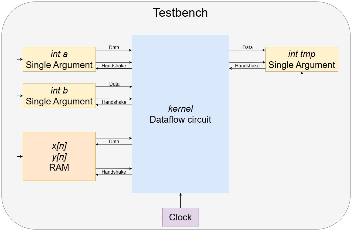
Auxiliary Processes
The first step of the testbench generation is to create a VHDL file called tb_<kernel_name>.vhd resp. a Verilog file tb_<kernel_name>.v which will contain all processes and instances needed to simulate the kernel. It is the top-level module for simulation.
Standard HDL boilerplate and processes for generating a clock signal, a reset signal and signals for starting and ending a simulation are written in Verilog or VHDL in tools/hls-verifier/include/HlsTb.h and are copied to the testbench file.
Constants
Constant values such as the clock period or reset latency can be defined with the function declareConstant(). The appropriate HDL implementation is then written to the testbench file.
Signals
Declaring signals that hold a value and are updated in procedural blocks need to be declared differently from signals that only connect two modules.
Therefore, there are two functions to declare signals: declareReg() and declareWire().
Verilog throws an error if the wrong type is selected. VHDL, on the other hand, does not make a distinction between the two types and both functions emit the same VHDL code.
Connections between two modules are declared using the function declareWire().
Single Argument
Single value input arguments (e.g. int a and int b) and output values (e.g. int tmp) are handled by the single argument module.
This module communicates by handshake signals with the dataflow circuit.
For every single valued input/output, a single argument module is instantiated from the template in tools/hls-verifier/resources/.
RAM
To load and store values from arrays (e.g. int x[n] and int y[n]), the testbench has a RAM module.
It is connected by data and handshake signals to the dataflow circuit.
The template is located in the same directory as the single argument.
Global Completion Signal
The simulation is finished when all output modules received their value. To collect all valid signals from the output instances the join_tb module is used.
Same as for the single argument and the RAM, the template is located in tools/hls-verifier/resources/.
Writing Output File
When the simulation is finished, the contents of the RAM and single argument modules are copied to the output file.
The HDL implementation for this process is given in hlsTb.h.
This concludes the testbench generation, and the circuit is now ready to be simulated.
Simulator Options
There are four different simulators currently supported by Dynamatic. ModelSim, Vivado Vitis, GHDL and Verilator. The first two can simulate both Verilog and VHDL files, where GHDL only works with VHDL and Verilator only with Verilog files.
warning
To use GHDL or Verilator, the correct HDL must be specified during Dynamatic’s write-hdl command.
Dynamatic’s simulate
The simulator can be selected with the flag --simulator during Dynamatic’s simulate command.
- ModelSim:
--simulator vsim - Vitis Vivado:
--simulator xsim - GHDL:
--simulator ghdl - Verilator:
--simulator verilator
Every simulator compiles all files in the /HDL_SRC directory and then starts the simulation with the testbench as top level module.
The implementation of the simulators is in tools/hls-verifier/include/Simulators.h. We will now briefly discuss every simulator.
ModelSim
When using ModelSim, Dynamatic creates a .do file with all necessary commands to elaborate, compile and execute the ModelSim simulation.
Dynamatic then passes this .do file when calling ModelSim.
Vivado Vitis
Dynamatic calls the xelab function of Vitis with the -R flag.
This elaborates and compiles the testbench and simulates the design.
GHDL
GHDL is executed using a shell script. All HDL source files are imported into GHDL, compiled and simulated.
Verilator
The Verilator main function is copied from tools/hls-verifier/resources/verilator_main.cpp to the working directory.
A shell script is used to call Verilator and run the simulation.
note
This is a proposal, and has not yet been implemented.
Operations which Add and Remove Extra Signals
As described in detail here, our Handshake IR uses a custom type system: each operand between two operations represents a handshake channel, enabling data to move through the circuit.
As a brief recap, an operand can either be a ControlType or a ChannelType. A ControlType operand is a channel for a control token, which is inherently dataless, while a ChannelType operand represents tokens carrying data.
Whether an operand is a ControlType or ChannelType, it can also carry extra signals: additional information present on tokens in this channel, separate to the normal data.
In order to enforce correct circuit semantics, all operations have strict type constraints specifying how tokens with extra signals may arrive and leave that operation (this is discussed in detail in the same link above).
Brief Recap of Rules
With only a few (truly exceptional) exceptions, operations must have the exact same extra signals on all inputs.
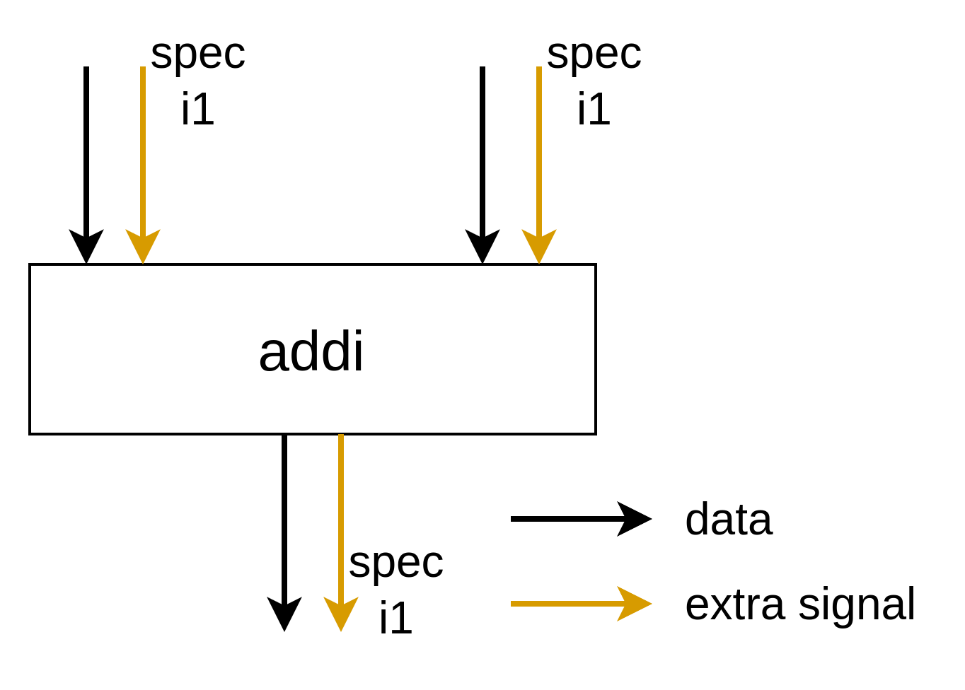
Load and Store operations are connected to our memory controllers, which currently do not support extra signals, and so we (currently) do not propagate these values to them.

As discussed in the full document on type verification, this could change in future if required, e.g. for out-of-order loads.
Operations which Add, Remove and Promote Extra Signals
We define an operation which adds an extra signal as an operation which receives token(s) lacking a specific extra signal, and outputs token(s) carrying that specific extra signal.
We define an operation which drops an extra signal as an operation which receives token(s) carrying a specific extra signal, and outputs token(s) lacking that specific extra signal.
We define an operation which promotes an extra signal as an operation which receives token(s) carrying a specific extra signal, and replaces the data value of that token with the value of that specific extra signal. This means the operation also outputs token(s) lacking that specific extra signal.
Due to concerns for modularity and composibility of extra signals, operations that add and remove extra signals should be introduced as rarely as possible, and as single-focusedly as possible.
If possible, the generic addSignal operation should be used:
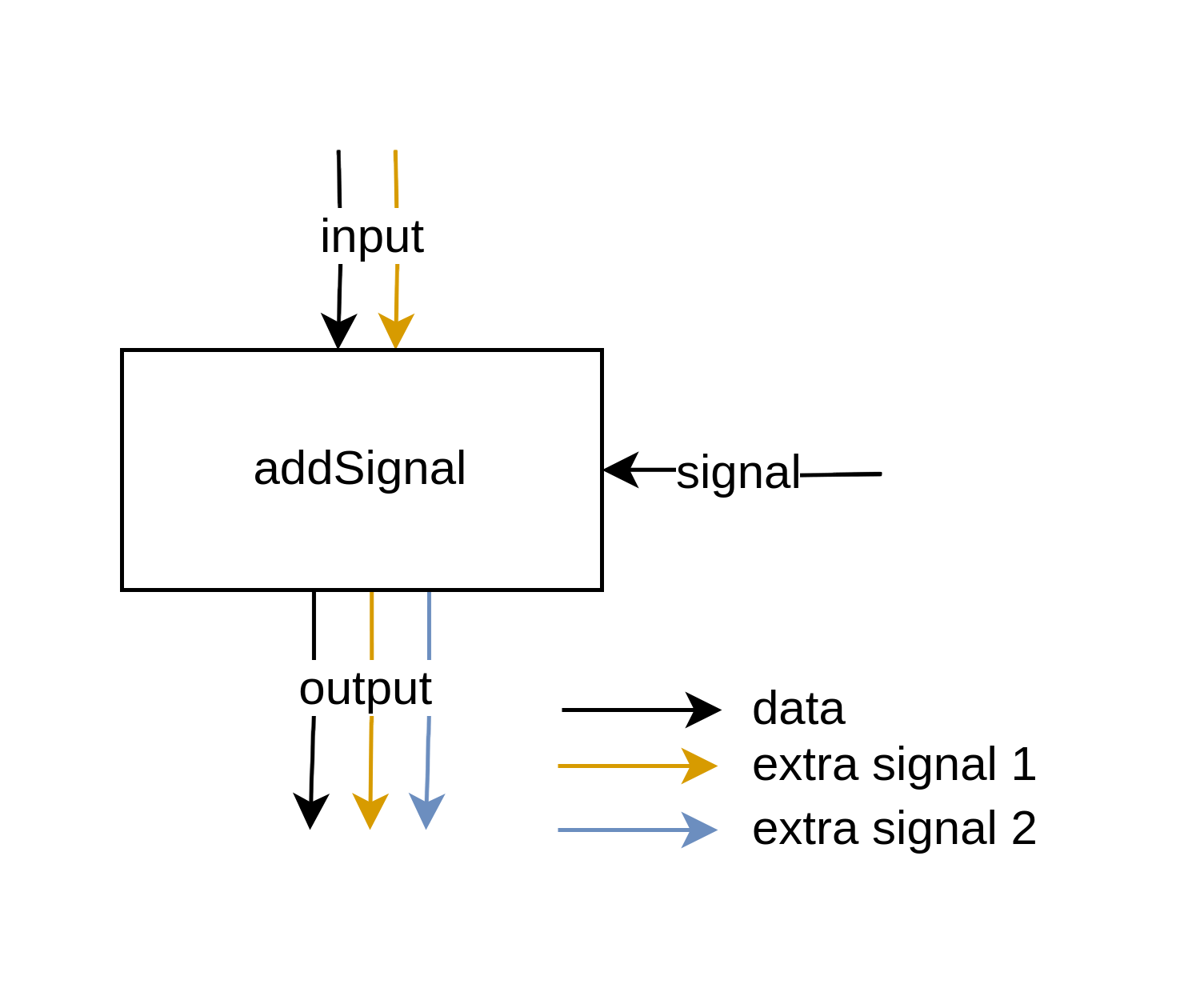
This separates how the value of the extra signal is generated from how the type of the input token is altered.
Only a single new extra signal can be added per addSignal operation.
Two extra signals parameters affect generation: the list of extra signals present at the input, and the added extra signal present at the output. These should be extracted from the type system just before the unit is generated, using an interface function present on the operation.
If possible, the generic dropSignal operation should be used:
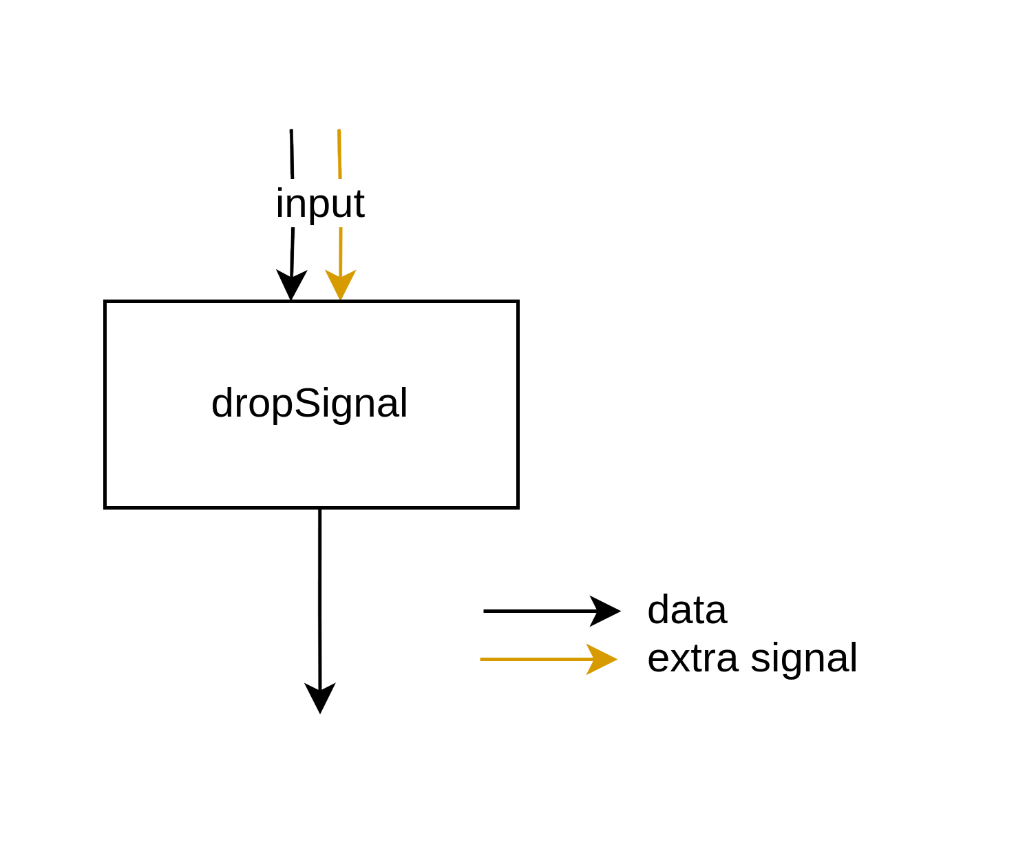
Only a single extra signal can be dropped per dropSignal operation.
Two extra signals parameters affect generation: the list of extra signals present at the output, and the dropped extra signal present at the input. These should be extracted from the type system just before the unit is generated, using an interface function present on the operation.
If possible, the generic promoteSignal operation should be used:
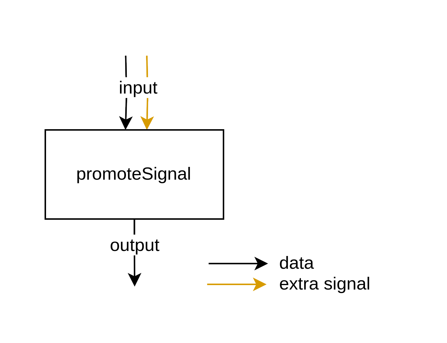
The promoteSignal operation promotes one extra signal to be the data signal, discarding the previous data signal.
Any additional extra signals, other than the promoted extra signal, are forwarded normally.
Two extra signals parameters affect generation: the list of extra signals present at the output, and the promoted extra signal present at the input. These should be extracted from the type system just before the unit is generated, using an interface function present on the operation.
Some Examples
Speculative Region
The below is a general description of a situation present in speculation, where incoming tokens must receive a spec bit before entering the speculative region:
When tokens must receive an extra signal on arriving in a region, and lose it when exiting that region, the region should begin and end with addSignal and dropSignal:
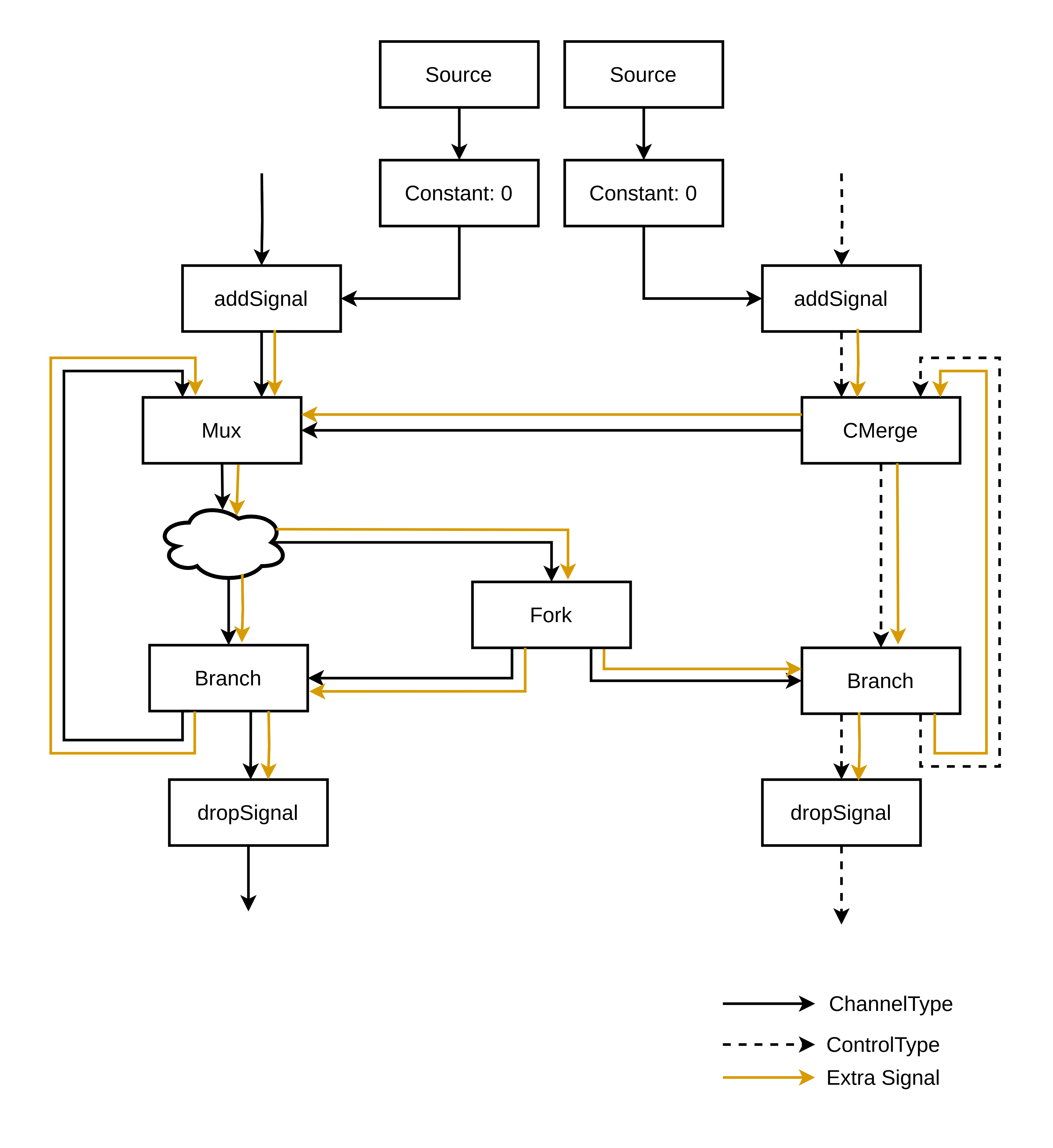
The incoming tokens may already have extra signals present, like so:
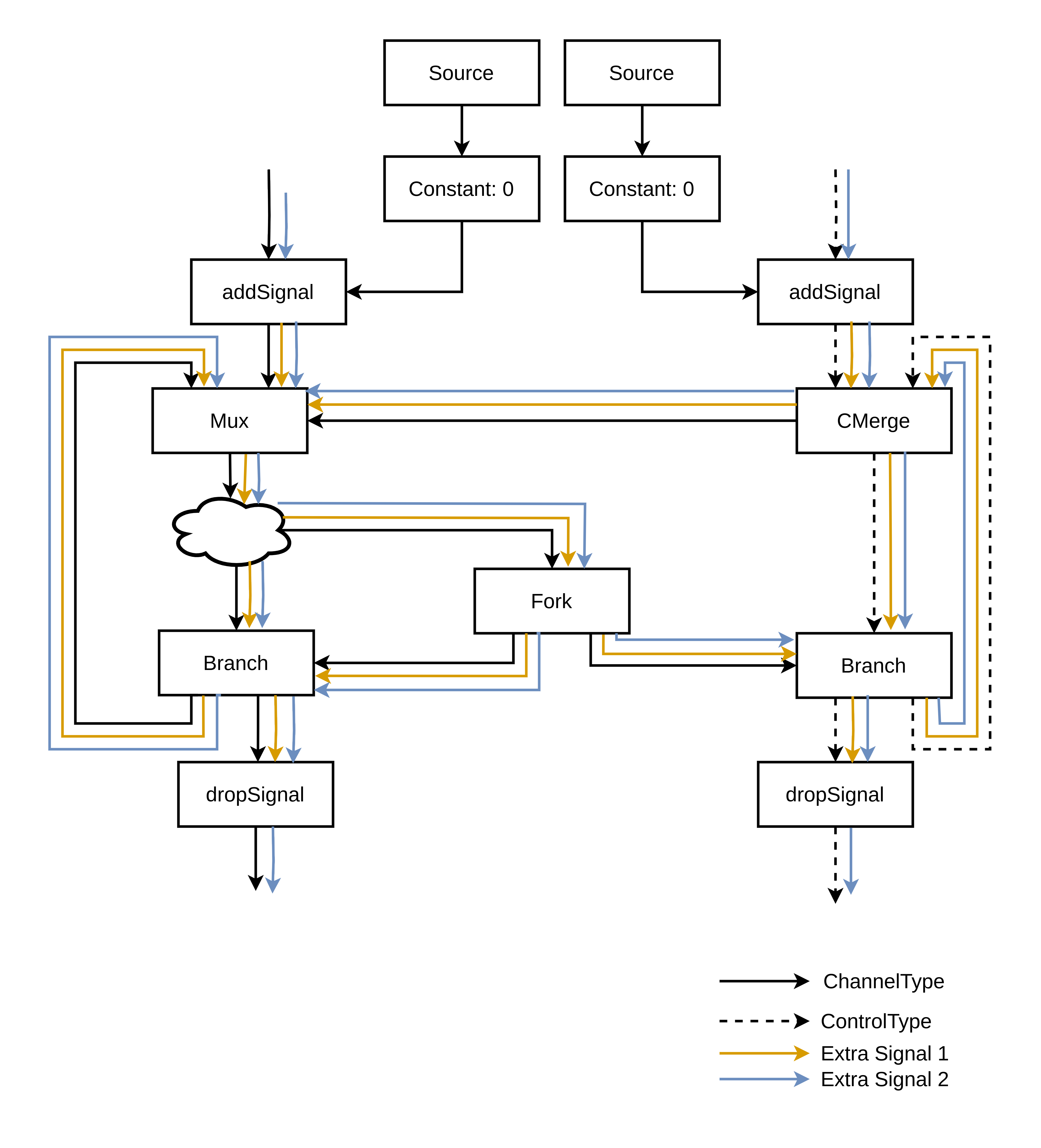
Speculating Branch
A speculating branch must branch the unit based on its spec bit, rather than the token’s data.
However, this example case applies to any unit which should branch based off an extra signal value.
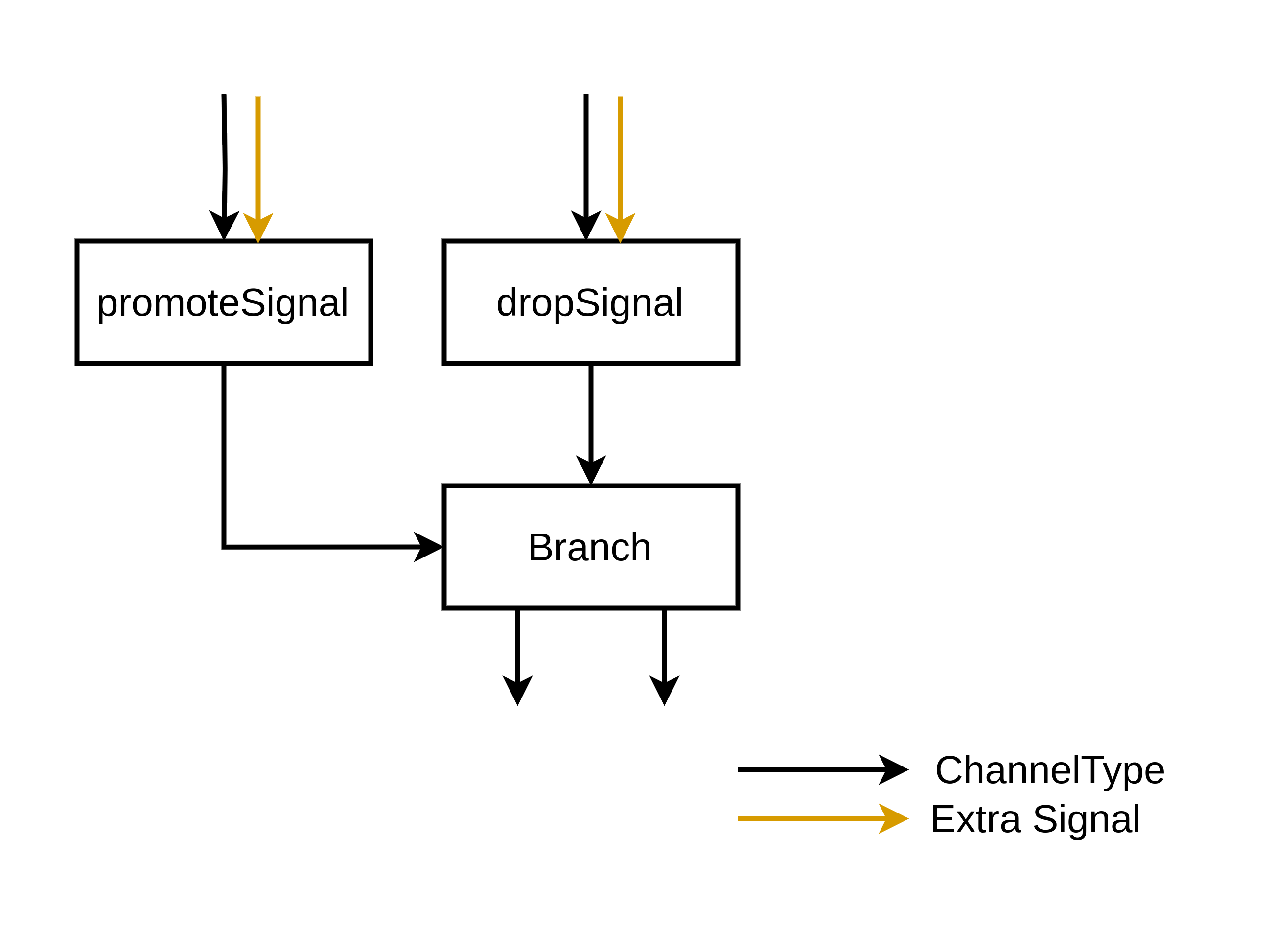
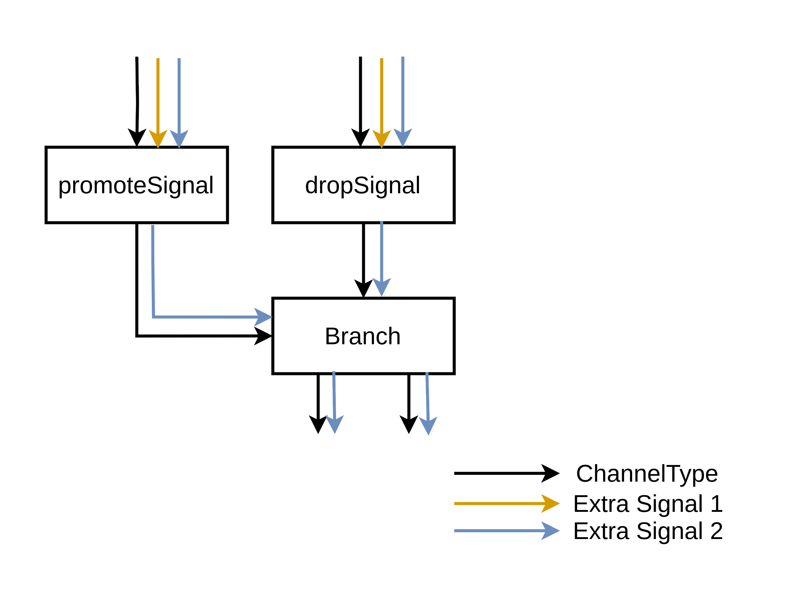
Aligning and Untagging for Out-Of-Order Execution
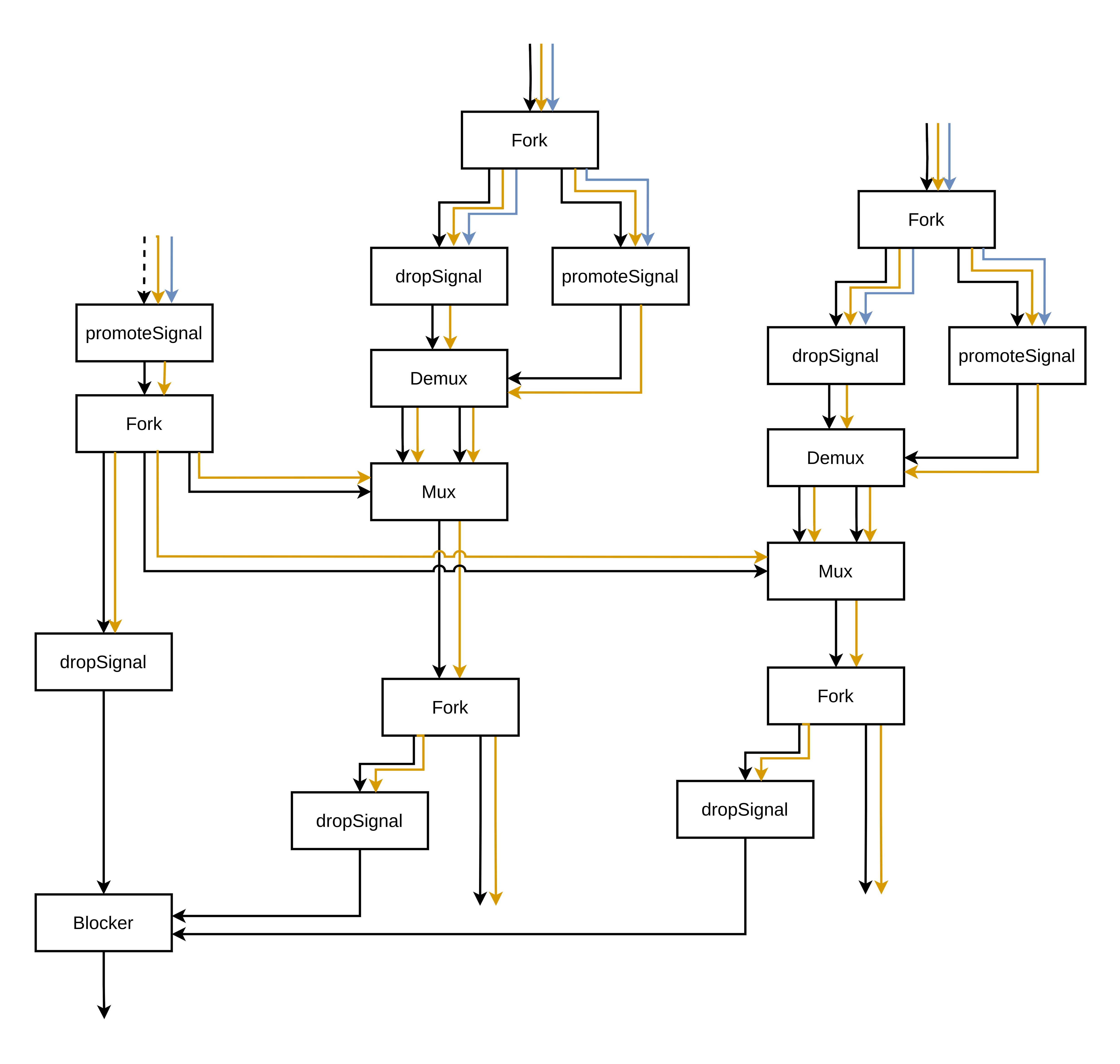
Circuit & Memory Interface
note
This is a proposed design change; it is not implemented yet.
The interface of Dynamatic-generated circuits has so far never been properly formalized; it is unclear what guarantees our circuits provide to the outside world, or even what the semantics of their top-level IO are. This design proposal aims to clarify these concerns and lay out clear invariants that all Dynamatic circuits must honor to allow their use as part of larger arbitrary circuits and the composition of multiple Dynamatic circuits together. This specification introduces the proposed interfaces by looking at our circuits at different levels of granularity.
- Circuit interface | Describes the semantics of our circuit’s top-level IO.
- Memory interface | Explains how we can implement standardized memory interfaces (e.g., AXI) from our ad-hoc ones.
- Internal implementation example | Example of how we may implement the circuits’ semantics internally.
Circuit interface
In this section, we look at the proposed interface for Dynamatic circuits. The figure below shows the composition of their top-level IO.

The inputs of a Dynamatic circuit are made up its arguments, a start signal, and of memory control inputs. Conversely, the outputs of a Dynamatic circuit are made up of its results, an end signal, and of memory control outputs. Finally, a Dynamatic circuits may have a list of ad-hoc memory interfaces, each made up of an arbitrary (and potentially differerent) bundle of signals. For design sanity, these memory interfaces should still be elastic even though their exact composition is up to the implementor.
important
We define a circuit execution as a single token (in the dataflow sense) being consumed on each of the circuit’s inputs, and a single token eventually being transmitted on each of the circuit’s outputs. After all output tokens have been transmitted—which necessarily happens after all inputs tokens have been consumed—we consider the execution to be completed. Dynamatic circuits may support streaming—i.e., concurrent executions on multiple sets of input tokens. In this case, Dynamatic circuits produce the set of output tokens associated to each execution in the order in which it consumed the sets of input tokens.
Dynamatic circuits guarantee that, after consuming a single token on each of their input ports, they will eventually produce a single token on each of their output ports; circuit executions are guaranteed to complete. However, they offer no guarantee on input consumption order across different input ports or output production order across different output ports.
start & end
start (displayed top-center in the figure) is a control-only input (downstream valid wire and uptream ready wire) that indicates to the Dynamatic circuit that it can start executing one time. Conversely, end (displayed bottom-center in the figure) is a control-only output that indicates that the Dynamatic circuit will eventually complete one execution.
Arguments & Results
A Dynamatic circuit may have 0 or more arguments ($N$ arguments displayed top-left in the figure) which are full dataflow inputs (downstream data bus and valid wire and uptream ready wire). Conversely, a Dynamatic circuit may have 0 or more results ($L$ results displayed bottom-left in the figure) which are full dataflow outputs. Note that the number of arguments and results may be different, and that the data-bus width of each argument input and result output may be different.
Memory Controls
A Dynamatic circuit may interact with 0 or more distinct memory regions. Interactions with each memory region is controlled independently by a pair of control-only ports, a mem_start input ($M$ memory control inputs displayed top-right in the figure) and mem_end output ($M$ memory control outputs displayed bottom-right in the figure). The mem_start input indicates to the Dynamatic circuit that it may start to make accesses to that memory region in the current circuit execution. Conversely, the mem_end output indicates that the Dynamatic circuit will not make any more accesses to the memory region in the current circuit execution.
note
The number of distinct memory regions that a Dynamatic circuit instantiates is not a direct function of the source code from which it was synthesized. The compiler is free to make optimizations or transformations as required. For convenience, Dynamatic still offers the option of simply assigning a distinct memory region to each array-typed argument in the source code.
Ad-hoc Memory Interfaces
A Dynamatic circuit connects to memory regions through ad-hoc memory interfaces ($M$ memory interfaces displayed right in the figure). These bidirectional ports may be different between memory regions; they carry the load/store requests back and forth between the Dynamatic circuit and the external memory region. Implementors are free to choose the exact signal bundles making up each memory interface.
important
While the specification imposes no restriction on these memory interfaces, it is good practice to always use some kind of elastic (e.g., latency-insensitive) interface to guaranteee compatibility with standardized latency-insensitive protocols such as AXI. Note that our current ad-hoc memory interfaces are not elastic, which should be fixed in the future.
Memory Interface
While the ad-hoc memory interfaces described above are very flexible by nature, users of Dynamatic circuits are likely to want to connect them to their design using standard memory interfaces and talk to them through standard communication protocols. To fulfill this requirement, Dynamatic should also be able to emit wrappers around its “core dataflow circuits” that simply convert every of its ad-hoc memory interface to a standard interface (such as AXI). The figure below shows how such a wrapper would look like.

The wrapper has exactly the same start, end, arguments, results, and memory control signals as the Dynamatic circuit it wraps. However, the Dynamatic circuit’s ad-hoc memory interfaces (double-sided arrows on the right of the inner box on the figure) get converted on-the-fly to standard memory interfaces (AXI displayed right in the figure). As a sanity check on any ad-hoc interface, it should always be possible and often easy to make load/store requests coming through them compliant with standard communication protocols.
Internal Implementation
This section hints at how one might implement the proposed interface in Dynamatic circuits. The goal is not to be extremely formal but rather to
- show that the proposed interface is sane and
- give a sense of how every port of the interface connects to the circuit’s architecture.
The figure below shows a possible internal implementation for Dynamatic circuits (note that the wrapper previously discussed is not shown in this picture). The rest of this section examines specific aspects of this rough schematic to give an intuition of how everything fits together.

start to end path
Recall the meaning of the start and end signals. start indicates that the circuit can start executing one time, while end indicates that the circuit will eventually complete one execution. Assuming a well-formed circuit that does not deadlock if all its inputs are provided, it follows that if the circuit starts an execution, it will eventually complete it. Therefore, start directly feeds into end.
Arguments to Results Path
The circuit’s arguments directly feed into the “internal circuit logic” block which eventually produces the circuit’s results. This block simply encapsulates the circuit-specific DFG (data-flow graph). In particular, it includes the circuit’s control network which is triggered by the “control synchronizer” shown below the start input. This synchronizer, in the simplest case, exists to ensure that only one set of input tokens is “circulating” inside the circuit logic at any given time. The synchronizer determines when the circuit starts an execution by looking at both the start input (indicating that we should at some point start executing with new inputs) and at the “exit block reached” signal coming from the circuit (indicating that a potential previous execution of the circuit has completed).
Memory Path
The schematic only shows the internal connectivity for a single memory region (mem2) for readability purposes. The connectivity for other memory regions may be assumed to be identical.
Internally, memory accesses for each memory region are issued by the internal circuit logic to an internal memory controller (e.g, LSQ), which then forwards these requests to an external memory through its associated ad-hoc memory interface; all of these communication channels are handshaked. The “memory synchronizer” shown below the mem2_start input informs the memory controller of when it is allowed to make memory requests through its interface. It makes that determination using a combination of the start input (indicating that the circuit should execute), the mem2_start input (indicating that accesses to the specific memory region are allowed), and of the memory controller’s own termination signal (indicating that any potential previous execution of the circuit will no longer make accesses to the region). The latter also feeds mem2_end.
An unused memory region may be ellided from the circuit interface entirely.
Type System
note
This is a proposed design change; it is not implemented yet.
Currently, at the Handshake IR level, all SSA values are implicitly assumed to represent dataflow channels, even when their type seems to denote a simple “raw” signal. More accurately, the handshake::FuncOp MLIR operation—which maps down from the original C kernel and eventually ends up as the top-level RTL module representing the kernel—provides implicit Handshake semantics to all SSA values defined within its regions.
For example, consider a trivial C kernel.
int adder(int a, int b) { return a + b; }
At the Handshake level, the IR that Dynamatic generates for this kernel would like as follows (some details unimportant in the context of this proposal are omitted for brevity).
handshake.func @adder(%a: i32, %b: i32, %start: none) -> i32  {
    %add = arith.addi %a, %b : i32
    %ret = handshake.return %add : i32
    handshake.end %ret : i32
}
Each i32-typed SSA value in this IR represents in fact a dataflow channel with a 32-bit data bus (which should be interpreted as an integer). Also note that control-only dataflow channel (with no data bus) are somewhat special-cased in the current type system by using the standard MLIR NoneType (written as none) in the IR. While this may be a questionnable design decision in the first place (the i0 type, which is legal in MLIR, could be conceived as a better choice), it is not fundamentally important for this proposal.
The Problem
On one hand, implicit dataflow semantics within Handshake functions have the advantage of yielding neat-looking IRs that do not bother to deal with an explicit parametric “dataflow type” repeated everywhere. On the other hand, it also prevents us from mixing regular dataflow channels (downstream data bus, downstream valid wire, and upstream ready wire) with any other kind of signal bundle.
- On one side, “raw” un-handshaked signals would look indistinguishable from regular dataflow channels in the IR. If a dataflow channel with a 32-bit data bus is represented using
i32, then no existing type can represent a 32-bit data bus without the valid/ready signal bundle. Raw signals could be useful, for example, for any kind of partial circuit rigidification, where some channels that provably do not need handshake semantics could drop their valid/ready bundle and only be represented as a single data bus. - On the other side, adding extra signals to some dataflow channels that may need to carry additional information around is also impossible modulo addition of a new parametric type. For example, speculation bits or thread tags cannot currently be modeled by this simple type system.
While MLIR attributes attached to operations whose adjacent channels are “special” (either because they drop handshake semantics or add extra signals) could potentially be a solution to the issue, we argue that it would be cumbersome to work with and error-prone for the following reasons.
- MLIR treats custom attribute opaquely, and therefore cannot automatically verify that they make any sense in any given context. We would have to define complex verification logic ourselves and think of verifying IR sanity every time we transform it.
- Attributes heavily clutter the IR, making it harder to look at whenever many operations possess (potentially complex) custom attributes. This hinders debuggability since it is sometimes useful to look directly at the serialized IR to understand what a pass inputs or outputs.
Proposed Solution
New Types
We argue that the only way to obtain the flexibility outlined above is to
- make dataflow semantics explicit in Handshake functions through the introduction of custom IR types, and
- use MLIR’s flexible and customizable type system to automatically check for IR sanity at all times.
We propose to add two new types to the IR to enable us to reliably model our use cases inside Handshake-level IR.
- A nonparametric type to model control-only tokens which lowers to a bundle made up of a downstream valid wire and upstream ready wire. This
handshake::ControlTypetype would serialize tocontrolinside the IR. - A parametric type to model dataflow channels with an arbitrary data type and optional extra signals. In their most basic form, SSA values of this type would be a composition of an arbitrary “raw-typed” SSA value (e.g.,
i32) and of acontrol-typed SSA value. It follows that values of this type, in their basic form, would lower to a bundle made up of a downstream data bus of a specific bitwidth plus what thecontrol-typed SSA value lowered to (valid and ready wires). Optionally, this type could also hold extra “raw-typed” signals (e.g., speculation bits, thread tags) that would lower to downstream or upstream buses of corresponding widths. Thishandshake::ChannelTypetype would serialize tochannel<data-type, {optional-extra-types}>inside the IR.
Considering again our initial simple example, it seems that the proposed changes would make the IR look identical modulo cosmetic type changes.
handshake.func @adder(%a: channel<i32>, %b: channel<i32>, %start: control) -> channel<i32>  {
    %add_result = arith.addi %a, %b : channel<i32>
    %ret = handshake.return %add_result : channel<i32>
    handshake.end %ret : channel<i32>
}
However, this in fact would be rejected by MLIR. The problem is that the standard MLIR operation representing the addition (arith.addi) expects operands of a raw integer-like type, as opposed to some custom data-type it does not know (i.e., channel<i32>). This in fact may have been one of the motivations behind the implicit dataflow semantic design assumption in Handshake; all operations from the standard arith and math dialects expect raw integer or floating-point types (depending on the specific operation) and cannot consequently accept custom types like the one we are proposing here. We will therefore need to redefine the standard arithmetic and mathematical operations within Handshake to support our custom data types. The IR would look identical as above except for the name of the dialect prefixing addi.
handshake.func @adder(%a: channel<i32>, %b: channel<i32>, %start: control) -> channel<i32>  {
    %add_result = handshake.addi %a, %b : channel<i32>
    %ret = handshake.return %add_result : channel<i32>
    handshake.end %ret : channel<i32>
}
New Operations
Occasionaly, we will want to unbundle channel-typed SSA values into their individual signals and later recombine the individual components into a single channel-typed SSA value. We propose to introduce two new operations to fulfill this requirement.
- An unbundling operation (
handshake::UnbundleOp) which generally breaks down its channel-typed SSA operand into its individual components, which it produces as separate SSA results. - A converse bundling operation (
handshake::BundleOp) which generally combines multiple raw-typed SSA operands and combines them into a single channel-typed SSA value which it produces as a single SSA result.
We include a simple example below (see the next subsection for more complex use cases).
// Breaking down a simple 32-bit dataflow channel into its individual
// control and data components, then rebundling it
%channel = ... : channel<i32>
%control, %data = handshake.unbundle %channel : control, i32
%channelAgain = handshake.bundle %control, %data : channel<i32>
Extra Signal Handling
To support the use case where extra signals need to be carried on some dataflow channel (e.g., speculation bits, thread tags), the handshake::ChannelType needs to be flexible enough to model an arbitrary number of extra raw data-types (in addition to the “regular” data-type). In order to prepare for future use cases, each extra signal should also be characterized by its direction, either downstream or upstream. Extra signals may also optionally declare unique names to refer themselves by, allowing client code to more easily query for a specifc signal in complex channels.
Below are a few MLIR serialization examples for dataflow channels with extra signals.
// A basic channel with 32-bit integer data and no extra signal
%channel = ... : channel<i32>

// -----

// A channel with 32-bit integer data and an extra unnamed 1-bit signal (e.g., a
// speculation bit) going downstream
%channel = ... : channel<i32, [i1]>

// -----

// A channel with 32-bit integer data and two extra named thread tags,
// respectively of 2-bit width and 4-bit width, both going downstream
%channel = ... : channel<i32, [tag1: i2, tag2: i4]>

// -----

// A channel with 32-bit integer data and an extra 1-bit signal going upstream,
// as indicated by the "(U)"; extra signals are by default downstream (most
// common use case) so they get no such annotation
%channel = ... : channel<i32, [otherReady: (U) i1]>
The unbundling and bundling operations would also unbundle and bundle, respectively, all the extra signals together with the raw data bus and control-only token.
// Multiple thread tags example from above
%channel = ... : channel<i32, [tag1: i2, tag2: i4]>

// Unbundle into control-only token and all individual signals
%control, %data, %tag1, %tag2 = handshake.unbundle %channel : control, i32, i2, i4

// Bundle to get back the original channel
%bundled = handshake.bundle %control, %data [%tag1, %tag2] : channel<i32, [tag1: i2, tag2: i4]>

// -----

// Upstream extra signal example from above
%channel = ... : channel<i32, [otherReady: (U) i1]>

// Unbundle into control-only token and raw data; note that, because the extra
// signal is going upstream, it is an input of the unbundling operation instead
// of an output
%control, %data = handshake.unbundle %channel, %otherReady : control, i32

// Bundle to get back the original channel; note that, because the extra signal
// is going upstream, it is an output of the bundling operation instead of an
// input
%bundled, %otherReady = handshake.bundle %control, %data : channel<i32, [otherReady: (U) i1]>

// -----

// Control-typed values can be further unbundled into their individual signals
%control = ... : control
%valid = handshake.unbundle %control, %ready : i1
%controlAgain, %ready = handshake.bundle %valid : control, i1
Most operations accepting channel-typed SSA operands will likely not care for these extra signals and will follow some sort of simple forwarding behavior for them. It is likely that pairs of specific Handshake operations will care to add/remove certain types of extra signals between their operands and results. For example, in the speculation use case, the specific operation marking the beginning of a speculative region would take care of adding an extra 1-bit signal to its operand’s specific channel-type. Conversely, the special operation marking the end of the speculative region would take care of removing the extra 1-bit signal from its operand’s specific channel-type.
Going further, if multiple regions requiring extra signals were ever nested within each other, it is likely that adding/removing extra signals in a stack-like fashion would suffice to achieve correct behavior. However, if that is insufficient and extra signals were not necessarily removed at the same rate or in the exact reverse order in which they were added, then the unique extra signal names could serve as identifiers for the specific signals that a signal-removing unit should care about removing.
Discussion
In this section we try to alleviate potential concerns with the proposed change and discuss the latter’s impact on other parts of Dynamatic.
Type Checking
Using MLIR’s type system to model the exact nature of each channel in our circuits makes us benefit from MLIR’s existing type management and verification infrastructure. We will be able to cleanly define and check for custom type checking rules on each operation type, ensuring that the relationships between operand and result types always makes sense; all the while permitting our operations to handle an infinite number of variations of our parametric types.
For example, the integer addition operation (handshake.addi) would check that its two operands and result have the same type. Furthermore, this type would only be required to be a channel with a non-zero-width integer type.
// Valid
%addOprd1, %addOprd2 = ... : channel<i32>
%addResult = handshake.addi %addOprd1, %addOprd2 : channel<i32>

// -----

// Invalid, data type has 0 width
%addOprd1, %addOprd2 = ... : channel<i0>
%addResult = handshake.addi %addOprd1, %addOprd2 : channel<i0>
IR Complexity
Despite the added complexity introduced by our parametric channel type, the representation of core dataflow components (e.g., merges and branches) would remain structurally identical beyond cosmetic type name changes.
// Current implementation
%mergeOprd1 = ... : none
%mergeOprd2 = ... : none
%mergeResult, %index = handshake.control_merge %mergeOprd1, %mergeOprd2 : none, i1

%muxOprd1 = ... : i32
%muxOprd2 = ... : i32
%muxResult = handshake.mux %index [%muxOprd1, %muxOprd2] : i32

// -----

// With proposed changes
%mergeOprd1 = ... : control
%mergeOprd2 = ... : control
%mergeResult, %index = handshake.control_merge %mergeOprd1, %mergeOprd2 : control, channel<i1>

%muxOprd1 = ... : channel<i32>
%muxOprd2 = ... : channel<i32>
%muxResult = handshake.mux %index [%muxOprd1, %muxOprd2] : channel<i1>, channel<i32>

// -----

// No extra operations when extra signals are present
%mergeOprd1 = ... : control
%mergeOprd2 = ... : control
%mergeResult, %index = handshake.control_merge %mergeOprd1, %mergeOprd2 : control, channel<i1>

%muxOprd1 = ... : channel<i32, [i2, i4]>
%muxOprd2 = ... : channel<i32, [i2, i4]>
%muxResult = handshake.mux %index [%muxOprd1, %muxOprd2] : channel<i1>, channel<i32, [i2, i4]>
Backend Changes
The support for “nonstandard” channels in the IR means that we have to match this support in our RTL backend. Indeed, most current RTL components take the data bus’s bitwidth as an RTL parameter. This is no longer sufficient when dataflow channels can carry extra downstream or upstream signals, which must somehow be encoded in the RTL parameters of numerous core dataflow components (e.g., all merge-like and branch-like components). Complex channels will need to become encodable as RTL parameters for the underlying RTL implementations to be concretized correctly. It is basically a given that generic RTL implementations which we largely rely on today will not be sufficient, and that the design change will require us moving to RTL generators for most core dataflow components. Alternatively, we could use a form of signal composition (see below) to narrow down the amount of channel types our components have to support.
Signal Compositon
In some instances, it may be useful to compose all of a channel’s signals going in the same direction (downstream or upstream) together around operations that do not care about the actual content of their operands’ data buses (e.g., all data operands of merge-like and branch-like operations). This would allow us to expose to certain operations “regular” dataflow channels without extra signals; their exposed data buses would in fact be constituted of the actual data buses plus all extra downstream signals. Just before lowering to HW and then RTL (after applying all Handshake-level transformations and optimizations to the IR), we could run a signal-composition pass that would apply this transformation around specific dataflow components in order to make our backend’s life easier.
Considering again the last example with extra signals from the IR complexity subsection above, we could make our current generic mux implementation work with the new type system without modifications to the RTL.
%index = ... : channel<i1>
%muxOprd1 = ... : channel<i32, [i2, i4]>
%muxOprd2 = ... : channel<i32, [i2, i4]>

// Our current generic RTL mux implementation does not work because of the extra
// signals attached to the data operands' channels
%muxResult = handshake.mux %index [%muxOprd1, %muxOprd2] : channel<i1>, channel<i32, [i2, i4]>

// -----

// Same inputs as before
%index = ... : channel<i1>
%muxOprd1 = ... : channel<i32, [i2, i4]>
%muxOprd2 = ... : channel<i32, [i2, i4]>

// Compose data operands's extra signals with the data bus
%muxComposedOprd1 = handshake.compose %muxOprd1 : channel<i32, [i2, i4]> -> channel<i38>
%muxComposedOprd2 = handshake.compose %muxOprd2 : channel<i32, [i2, i4]> -> channel<i38>

// Our current generic RTL mux implementation would work out-of-the-box!
%muxComposedResult = handshake.mux %index [%muxComposedOprd1, %muxComposedOprd2] : channel<i1>, channel<i38>

// Most likely some operation down-the-line actually cares about the isolated
// extra signals, so undo handshake.compose's effect on the mux result
%muxResult = handshake.decompose %muxComposedResult : channel<i38> -> channel<i32, [i2, i4]>
The RTL implementations of the handshake.compose and handshake.decompose signals would be trivial and offload complexity from the dataflow components themselves, making the latter’s RTL implementations simpler and area smaller.
A similar yet slightly different composition behavior could help us simplify the RTL implementation of arithmetic operations—which would usually forward all extra signals between their operands and results—as well. In cases where it makes sense, we could compose all of the operands’ and results’ downstream extra signals into a single one that is still separate from the data signal, which arithmetic operations actually use. We could then design a (couple of) generic implementation(s) for these arithmetic operations that would work for all channel types, removing the need for a generator.
%addOprd1 = ... : channel<i32, [i2, i4, (U) i4, (U) i8]>
%addOprd2 = ... : channel<i32, [i2, i4, (U) i4, (U) i8]>

// Given the variability in the extra signals, this operation would require an
// RTL generator
%addResult = handshake.addi %addOprd1, %addOprd2 : channel<i32, [i2, i4, (U) i4, (U) i8]>

// -----

// Same inputs as before
%addOprd1 = ... : channel<i32, [i2, i4, (U) i4, (U) i8]>
%addOprd2 = ... : channel<i32, [i2, i4, (U) i4, (U) i8]>

// Compose all extra signals going in the same direction into a single one
%addComposedOprd1 = handshake.compose %addOprd1 : channel<i32, [i2, i4, (U) i4, (U) i8]>
                                                  -> channel<i32, [i6, (U) i12]>
%addComposedOprd2 = handshake.compose %addOprd2 : channel<i32, [i2, i4, (U) i4, (U) i8]>
                                                  -> channel<i32, [i6, (U) i12]>

// We could design a generic version of the adder that accepts a single
// downstream extra signal and a single upstream data signal
%addComposedResult = handshake.addi %addComposedOprd2, %addComposedOprd2 : channel<i32, [i6, (U) i12]>

// Decompose back into the original type
%addResult = handshake.decompose %addComposedResult : channel<i32, [i6, (U) i12]>
                                                      -> channel<i32, [i2, i4, (U) i4, (U) i8]>
Compiler Intrinsics
Wait
note
This is a proposed design change; it is not implemented yet.
There are many scenarios in which one may want to explicitly specify synchronization constraints between variables at the source code level and have Dynamatic circuits honor these temporal relations on its corresponding dataflow channels. In particular, this proposal focuses on a particular type of synchronization we call wait. Our goal here is to introduce a standard way for users to enforce the waiting relation between two source-level variables and provide insights as to how the compiler will treat the associated compiler intrinsic, ultimately resulting in a dataflow circuit honoring the relation.
Example
Consider the following pop_and_wait kernel.
// Pop from a FIFO identified by an integer.
// Note that the function has no body, so it will be treated as an external
// function by Dynamatic (the user is ultimately expected to provide a circuit
// for it to connect to the Dynamatic-generated circuit).
int pop(int queueID);

// Pop first two elements from the FIFO and return their difference.
int pop_and_wait(int queueID) {
  int x = pop(queueID);
  int y = pop(queueID);
  return x - y;
}
If this were to be executed on a CPU with a software implementation of pop, the two pop calls would happen naturally in the order in which they were specified in the code, yielding a correct kernel result every time. However, the ordering of the calls is no longer guaranteed in the world of dataflow circuits. Both calls are in the same basic block and have no explicit data dependency between them, meaning that Dynamatic is free to “execute them” in any order according to the availability of their (identical) operand and to the internal queue popping logic. If the second pop executes before the first one, then the kernel will produce the negation of its expected result. For reference, the Handshake-level IR for this piece of code might look something like the following.
handshake.func private @pop(channel<i32>, control) -> (i32, control)

handshake.func @pop_and_wait(%queueID: channel<i32>, %start: control) -> channel<i32> {
  %forkedQueueID:2  = fork [2] %queueID : channel<i32>
  %forkedStart:2    = fork [2] %start : channel<i32>
  %x, _             = instance @pop(%forkedQueueID#0, %forkedStart#0) : (channel<i32>, control) -> channel<i32>
  %y, _             = instance @pop(%forkedQueueID#1, %forkedStart#1) : (channel<i32>, control) -> channel<i32>
  %res              = arith.subi %x, %y : channel<i32>
  %output           = return %res : channel<i32>
  end %output : channel<i32>
}
Creating a Data Dependency
We need a way, in the source code, to tell Dynamatic that the second pop should always happen after the first has produced its result. One way to enforce this is to create a “fake” data dependency that makes the second use of queueID depend on x, the result of the first pop. We propose to represent this using a family of __wait compiler intrinsics. The pop_and_wait kernel may be rewritten as follows.
// Pop first two elements from the FIFO and return their difference.
int pop_and_wait(int queueID) {
  int x = pop(queueID);
  queueID = __wait_int(__int_to_token(x), queueID);
  int y = pop(queueID);
  return x - y;
}
__wait_int is a compiler intrinsic—a special function with a reserved name which Dynamatic will give special treatment too during compilation—that expresses the user’s desire that its return value (here queueID) only becomes valid (in the dataflow sense) when both of its arguments become valid in the corresponding dataflow circuit. The return value’s payload inherits the second arguments’s (here queueID) payload. This effectively creates a data dependency between x and queueID in between the two pops.
Intrinsic Prototypes
Supporting the family of __wait compiler intrinsics in source code amounts to adding the following function prototypes once to the main Dynamatic C header (that all kernels should include).
// Opaque token type
typedef int Token;

// Family of __wait intrinsics for all supported types
char      __wait_char(Token waitFor, char data);
short     __wait_short(Token waitFor, short data);
int       __wait_int(Token waitFor, int data);
unsigned  __wait_unsigned(Token waitFor, unsigned data);
float     __wait_float(Token waitFor, float data);
double    __wait_double(Token waitFor, double data);

// Family of conversion functions to "Token" type
Token     __char_to_token(char x);
Token     __short_to_token(short x);
Token     __int_to_token(int x);
Token     __unsigned_to_token(unsigned x);
Token     __float_to_token(float x);
Token     __double_to_token(double x);
The lack of support for function overloading in C forces us to have a collection of functions for all our supported types. The opaque Token type and its associated conversion functions (__*_to_token) allows us to have a unique type for the first argument of all __wait intrinsics, regardless of the payload’s type. Without it we would have had to define a __wait variant for each type combination in its two arguments or resort to illegal C value casts that either do not compile or yield convoluted IRs. Each __*_to_token conversion function in the source code yield a single additional IR operation which can easily be removed during the compilation flow.
Compiler Support
Our example kernel would lower to a very simple IR at the cf (control flow) level.
func.func @pop_and_wait(%queueID: i32) -> i32 {
  %x              = call @pop(%queueID) (i32) -> i32
  %firstPopToken  = call @__int_to_token(%firstPop) : (i32) -> i32
  %retQueueID     = call @__wait_int(%firstPopToken, %queueID) : (i32, i32) -> i32
  %y              = call @pop(%retQueueID) : (i32) -> i32
  %res            = arith.subi %x, %y : i32
  return %res : i32
}

func.func private @pop(i32) -> i32
func.func private @__wait_int(i32, i32) -> i32
func.func private @__int_to_token(i32) -> i32
During conversion to Handshake, Dynamatic would recognize the intrinsic functions via their name and yield appropriate IR constructs to implement the desired behavior.
handshake.func @pop_and_wait(%queueID: channel<i32>, %start: control) -> (channel<i32>, control) {
  %forkedQueueID:2  = fork [2] %queueID : channel<i32>
  %forkedStart:3    = fork [2] %start : channel<i32>
  %x, _             = instance @pop(%forkedQueueID#0, %forkedStart#0) : (channel<i32>, control) -> channel<i32>
  %retQueueID       = wait %x, %forkedQueueID#1 : (channel<i32>, channel<i32>) -> channel<i32>
  %y, _             = instance @pop(%retQueueID, %forkedStart#1) : (channel<i32>, control) -> channel<i32>
  %res              = arith.subi %x, %y : channel<i32>
  %output           = return %res : channel<i32>
  end %output, %forkedStart#2 : channel<i32>, control
}

handshake.func private @pop(channel<i32>, control) -> (channel<i32>, control)
We hightlight two key intrinsic-related aspects of the cf-to-handshake conversion below.
- The call to
__int_to_tokenhas completely disappeared from the IR (both as an operation inside the@pop_and_waitfunction and as an external function declaration). As mentionned previously, this family of conversion functions only serves the purpose of source-level type-checking, and do not map to any specific behavior in the resulting dataflow circuit. - The call to
__wait_intwas replaced by a new Handshake operation calledwait, which implements the behavior we describe above. All__waitvariants can map to a single MLIR operation thanks to MLIR’s support for custom per-operation type-checking semantics. Note that the@__wait_intexternal function declaration is no longer part of the IR either.
Development
Documentation related to development and tooling.
MLIR LSP
The MLIR project includes an LSP server implementation that provides editor integration for editing MLIR assembly (diagnostics, documentation, autocomplete, ..)1. Because Dynamatic uses additional out-of-tree MLIR dialects (Dynamatic handshake, Dynamatic hw), we provide an extended version of this LSP server with these dialects registered.
This server is built automatically during the Dynamatic compilation flow, and can be found at ./bin/dynamatic-mlir-lsp-server once ready. Usage of this LSP is IDE-specific.
VSCode
TODO
NeoVim (lspconfig)
NVIM’s lspconfig2 provides integration for the normal MLIR lsp server. We recommend relying on this, and only conditionally overriding the cmd used to start the server if inside the Dynamatic folder hierarchy.
For example, this can be achieved by overriding the cmd of the LSP server when registering it:
lspconfig.mlir_lsp_server.setup({
    cmd = (function()
        local fallback = { "mlir_lsp_server" }

        local dynamatic_proj_path = vim.fs.find('dynamatic', { path = vim.fn.getcwd(), upward = true })[1]
        if not dynamatic_proj_path then return fallback end -- not in dynamatic

        local lsp_bin = dynamatic_proj_path .. "/bin/dynamatic-mlir-lsp-server"
        if not vim.uv.fs_stat(lsp_bin) then
            vim.notify("Dynamatic MLIR LSP does not exist.", vim.log.levels.WARN)
            return fallback
        end

        vim.notify("Using local MLIR LSP (" .. dynamatic_proj_path .. ")", vim.log.levels.INFO)
        return { lsp_bin }
    end)(),
    -- ...
})
Alternatively, you can add an lspconfig hook to override the server cmd during initialization. Note that this
hook must be registered before you use lspconfig to setup mlir_lsp_server.
lspconfig.util.on_setup = lspconfig.util.add_hook_before(lspconfig.util.on_setup, function(config)
    if config.name ~= "mlir_lsp_server" then return end -- other lsp

    local dynamatic_proj_path = vim.fs.find('dynamatic', { path = vim.fn.getcwd(), upward = true })[1]
    if not dynamatic_proj_path then return end -- not in dynamatic

    local lsp_bin = dynamatic_proj_path .. "/bin/dynamatic-mlir-lsp-server"
    if not vim.uv.fs_stat(lsp_bin) then
        vim.notify("Dynamatic MLIR LSP does not exist.", vim.log.levels.WARN)
        return
    end

    vim.notify("Using local MLIR LSP (" .. dynamatic_proj_path .. ")", vim.log.levels.INFO)
    config.cmd = { lsp_bin }
end)
lspconfig.mlir_lsp_server.setup({
    -- ...
})
Documentation
Dynamatic’s documentation is written in markdown, which is located in the ./docs folder.
It is rendered to an HTML web page using mdbook, which is hosted at https://epfl-lap.github.io/dynamatic/, automatically on every push to the main repository.
Compiling the Documentation
To render and view the documentation locally, please install mdbook, and the mdbook-alerts plugin
Optionally, you can install the mdbook-linkcheck backend, to check for broken links in the documentation.
Then, from the root of the repository run:
mdbook build: to compile the documentation to HTML.mdbook serve: to compile the documentation and host it on a local webserver. Navigate to the shown location (usually localhost:3000) to view the docs. The docs are automatically re-compiled when they are modified.
Adding a new page
The structure of the documentation page is determined by the ./docs/SUMMARY.md file.
If you add a new page, you must also list it in this file for it to show up.
Note that we try to mirror the documentation file structure in the ./docs folder and the actual documentation structure.
Buffering
Overview
This document describes the current buffer placement infrastructure in Dynamatic.
Dynamatic represents dataflow circuit buffers using the handshake::BufferOp operation in the MLIR Handshake dialect. This operation has a single operand and a single result, representing the buffer’s input and output ends.
The document provides:
- A description of the
handshake::BufferOpoperation and its key attributes - An overview of available buffer types
- Mapping strategies from MILP results to buffer types
- Additional buffering heuristics (also referenced in code comments)
- Clarification of RTL backend behavior
It serves as a unified reference for buffer-related logic in Dynamatic.
Buffer Operation Representation
The handshake::BufferOp operation takes several attributes that characterize the buffer:
BUFFER_TYPE: Specifies the type of buffer implementation to useTIMING: A timing attribute that specifies cycle latencies on various signal pathsNUM_SLOTS: A strictly positive integer denoting the number of slots the buffer has (i.e., the maximum number of dataflow tokens it can hold concurrently)
In its textual representation, the handshake::BufferOp operation appears as follows:
%dataOut = handshake.buffer %dataIn {hw.parameters = {BUFFER_TYPE = "FIFO_BREAK_DV", NUM_SLOTS = 4 : ui32, TIMING = #handshake<timing {D: 1, V: 1, R: 0}>}} : <i1>
Here %dataIn is the buffer’s operand SSA value (the input dataflow channel) and %dataOut is the buffer’s result SSA value (the output dataflow channel).
Timing Information
The TIMING attribute specifies how many cycles of latency the buffer introduces on each handshake signal: data (D), valid (V), and ready (R).
D: 1means 1-cycle latency on the data pathR: 0means no latency on the ready path
Buffer Types
Each buffer type corresponds to a specific RTL backend HDL module with different timing, throughput and area characteristics. The Legacy name refers to the name previously used in the source code or HDL module before the standardized buffer type naming was introduced.
| Type name | Legacy name | Latency | Timing |
|---|---|---|---|
ONE_SLOT_BREAK_DV | OEHB | Data: 1, Valid: 1, Ready: 0 | Break: D, V; Bypass: R |
ONE_SLOT_BREAK_R | TEHB | Data: 0, Valid: 0, Ready: 1 | Break: R; Bypass: D, V |
ONE_SLOT_BREAK_DVR | N/A | Data: 1, Valid: 1, Ready: 1 | Break: D, V, R |
FIFO_BREAK_DV | elastic_fifo_inner | Data: 1, Valid: 1, Ready: 0 | Break: D, V; Bypass: R |
FIFO_BREAK_NONE | TFIFO | Data: 0, Valid: 0, Ready: 0 | Bypass: D, V, R |
SHIFT_REG_BREAK_DV | N/A | Data: 1, Valid: 1, Ready: 0 | Break: D, V; Bypass: R |
Additional notes on modeling and usage of the buffer types listed above:
-
Equivalent combinations:
Existing algorithms (FPGA20, FPL22, CostAware) do not distinguish between a singleFIFO_BREAK_DVand the combination ofONE_SLOT_BREAK_DVwithFIFO_BREAK_NONE, even though the two differ in both timing behavior and area cost.
Specifically, the algorithms treat ann-slotFIFO_BREAK_DVas equivalent to a1-slotONE_SLOT_BREAK_DVfollowed by ann-1-slotFIFO_BREAK_NONE. -
Control granularity:
InONE_SLOT_BREAK_DV, each slot has its own handshake control, so slots accept or stall inputs independently.
In contrast, all slots inSHIFT_REG_BREAK_DVshare a single handshake control signal and thus accept or stall inputs together. -
Composability:
All six buffer types can be used together in a channel to handle various needs.- For the first three types (
ONE_SLOT_BREAK_DV,ONE_SLOT_BREAK_R,ONE_SLOT_BREAK_DVR), multiple modules can be chained to provide more slots. - For the last three types (
FIFO_BREAK_DV,FIFO_BREAK_NONE,SHIFT_REG_BREAK_DV), multiple slots are supported within their module parameters, so they need not be chained.
- For the first three types (
-
Builder assertion:
An assertion is placed in theBufferOpbuilder to ensure that if the buffer type isONE_SLOT, thenNUM_SLOTS == 1.
Mapping MILP Results to Buffer Types
In MILP-based buffer placement (Mixed Integer Linear Programming), such as those used in the FPGA20 and FPL22 algorithms, the optimization model determines:
- Which signal paths (D, V, R) are broken by the buffer on each channel
- The number of buffer slots (
numslot) for the buffer on each channel
The MILP does not model or select buffer types directly. Instead, buffer types are assigned afterward based on the MILP results, using mapping logic specific to each buffer placement algorithm:
FPGA20 Buffers
1. If breaking DV:
   Map to ONE_SLOT_BREAK_DV + (numslot - 1) * FIFO_BREAK_NONE.

2. If breaking none:
   Map to numslot * FIFO_BREAK_NONE.
FPL22 Buffers
1. If breaking DV & R:
   When numslot = 1, map to ONE_SLOT_BREAK_DVR;
   When numslot > 1, map to ONE_SLOT_BREAK_DV + (numslot - 2) * FIFO_BREAK_NONE + ONE_SLOT_BREAK_R.

2. If only breaking DV:
   Map to ONE_SLOT_BREAK_DV + (numslot - 1) * FIFO_BREAK_NONE.

3. If only breaking R:
   Map to ONE_SLOT_BREAK_R + (numslot - 1) * FIFO_BREAK_NONE.

4. If breaking none:
   Map to numslot * FIFO_BREAK_NONE.
Additional Buffering Heuristics
In addition to the MILP formulation and its buffer type mapping logic, Dynamatic applies a number of additional buffering heuristics, either encoded as extra constraints within the MILP or applied during buffer placement, to ensure correctness and improve circuit performance.
The following rules are currently implemented:
Buffering before LSQ Memory Ops to Mitigate Latency Asymmetry
In the current dataflow circuit, we observe the following structure:
Store issues memory writes and sends a token to the LSQ after argument dispatch.
LSQ uses group-based allocation, triggered by CMerge, to dynamically schedule memory accesses.
The problem is that, the Store can only forward its token to LSQ one cycle after the CMerge-side token triggers allocation. Since the store path lacks a buffer, this creates an asymmetric latency across the two sides. As a result, back pressure from the store side propagates upstream and causes II += 1 in some benchmarks.
Currently, our buffer placement algorithm does not account for the group allocation latency and the dependency of Store on that allocation.
The same latency asymmetry applies to Load operations, which also depend on LSQ group allocation.
To mitigate this issue, a minimum slot number is enforced at the input of Store and Load operations connected to LSQs. This serves as a temporary workaround until a better solution is developed.
Breaking Ready Paths after Merge-like Operations (FPGA20)
In the FPGA20 buffer placement algorithm, buffers only break the data and valid paths. To prevent combinational cycles on ready paths, ready-breaking buffers are inserted after merge-like operations (e.g., Mux, Merge) if the output channel is part of a cycle.
Buffering after Merge Ops to Prevent Token Reordering
For any MergeOp with multiple inputs, at least one slot is required on each output if the output channel is part of a cycle. This prevents token reordering and ensures correct circuit behavior.
The following example illustrates the issue:
In this figure:
- the token enters the loop through the left input of the merge
- there is no buffer before the merge and the first eager fork
Suppose the first eager fork is backpressured by one of its outputs, but not backpressured by the output that circulates the token back to the right input of the merge. Then, there is a risk that the fork duplicates the token and passes it to the right input of the merge while there is still an incoming token to the left input of the merge. And merge might reorder these two tokens.
But if we always make sure that there is a buffer in between the merge and the first eagerfork below it, there is no such problem.
Unbufferizable Channels
- Memory reference arguments are not real edges in the graph and are excluded from buffering.
- Ports of memory interface operations are also unbufferizable.
These channels are skipped during buffer placement.
Buffering on LSQ Control Paths
- Fork outputs leading to other group allocations of the same LSQ must have a buffer that breaks data/valid paths.
- Other fork outputs must have a buffer that does not break data/valid paths.
See this paper for background.
RTL Generation
The RTL backend selects buffer implementations based on the BUFFER_TYPE attribute in each handshake::BufferOp. This determines the HDL module to instantiate. The NUM_SLOTS attribute is passed as a generic parameter.
The backend does not use TIMING when generating RTL. Latency information is kept in the IR for buffer placement only.
This design simplifies support for new buffer types: adding a new module and registering it in the JSON file is sufficient.
Code Structure
The following is the code structure in the BufferPlacement folder:
- BufferPlacementMILP.cpp: It contains all the functions and variables that are essential to instantiate variables and constraints in the MILP. All constraint instantiation functions should be defined in this file.
- BufferingSupport.cpp: It contains all the utilities for the files in this folder.
- CFDFC.cpp: It contains the functions generating the MILP formulation used to identify CFDFC in the dataflow circuit.
- CostAwareBuffer.cpp: It contains the functions generating the MILP formulation for cost-aware buffer placement.
- FPGA20Buffers.cpp: It contains the functions generating the MILP formulation for FPGA20 buffer placement.
- FPL22Buffers.cpp: It contains the functions generating the MILP formulation for FPL22 buffer placement.
- HandshakePlaceBuffers.cpp: It contains the main functions that orchestrate which buffer placement to call and the correct instantiation of buffers in the dataflow circuit.
- HandshakeSetBufferingProperties.cpp: It sets specific buffering properties for particular dataflow units (i.e., LSQ).
- MAPBUFBuffers.cpp: It contains the functions generating the MILP formulation for MapBuf buffer placement.
MapBuf
Overview
This file provides describes the MapBuf buffer placement algorithm. The algorithm is detailed in the paper MapBuf: Simultaneous Technology Mapping and Buffer Insertion for HLS Performance Optimization.
The document provides:
- Required compilation flags for running MapBuf
- Overview of the MILP constraint functions
- Delay characterization and propagation for carry-chains
- Results
File Structure
All MapBuf documentation is located under /docs/Specs/Buffering/MapBuf/, while the implementation files are found in the /experimental/lib/Support/ directory.
- blif_generator.py: A script that generates AIGs in BLIF using the HDL representations of dataflow units.
- BlifReader.cpp: It handles parsing and processing of BLIF files to convert them into internal data structures.
- CutlessMapping.cpp: It implements cut generation algorithm for technology mapping.
- SubjectGraph.cpp: It implements the core hardware-specific Subject Graph classes.
- BufferPlacementMILP.cpp: It contains all the functions and variables that are essential to instantiate variables and constraints in the MILP.
- MAPBUFBuffers.cpp: It contains the functions generating the MILP formulation for MapBuf buffer placement.
Flow of the Algorithm
The algorithm consists of 2 main parts, AIG generation and main buffer placement pass.
AIG Generation
To run MapBuf, BLIF files must first be generated. These can be created using the provided BLIF generation script or obtained from the dataflow-aig-library submodule.
Main Buffer Placement Pass
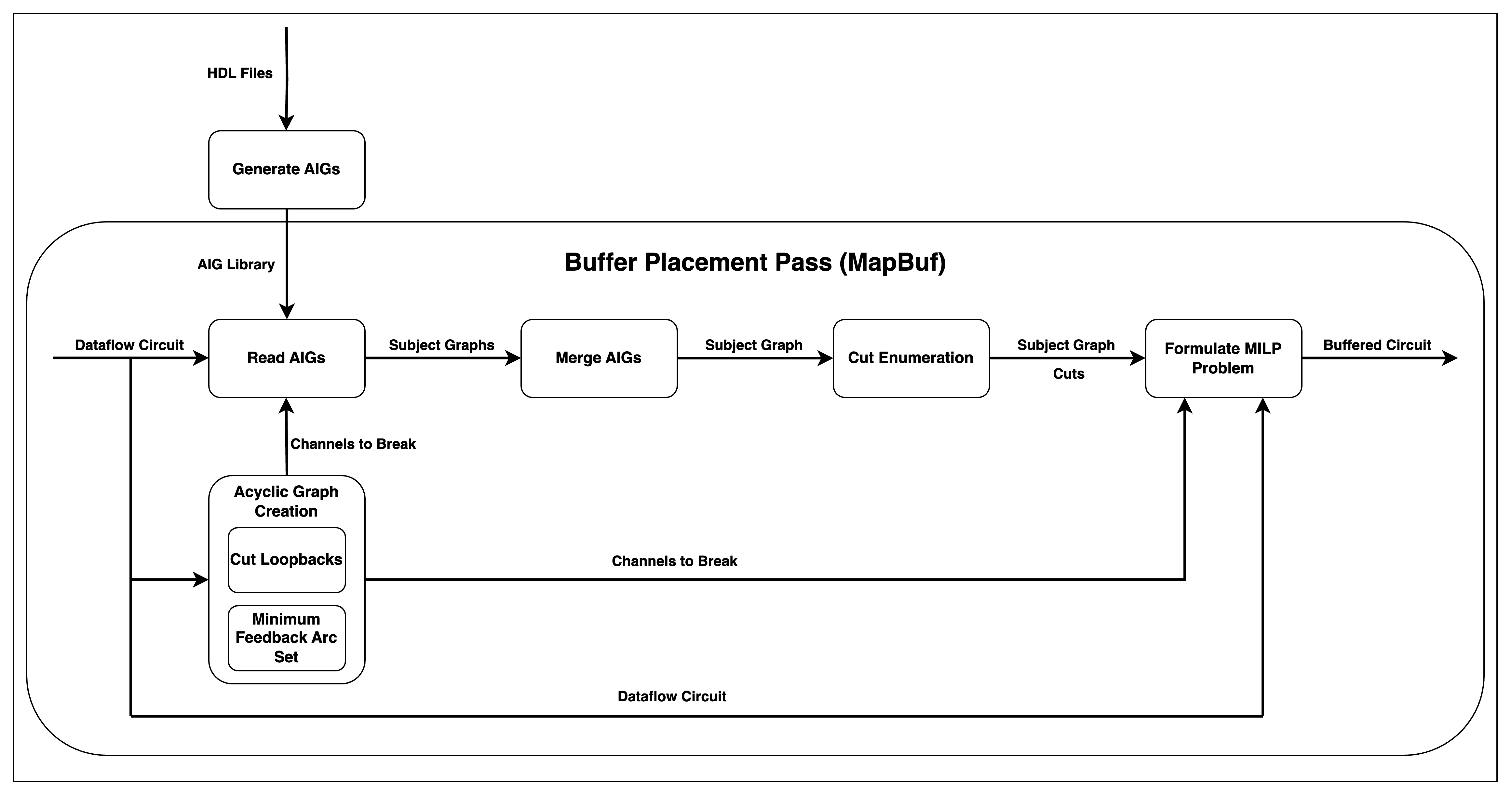
- Acyclic Graph Creation
- Takes the dataflow circuit and finds which channels need to be broken in order to have an acyclic graph.
- Such channels can be found by either Cut Loopbacks method or Minimum Feedback Arc Set method, implemented in BufferPlacementMILP.cpp.
- Read AIGs
- Takes the dataflow circuit and reads the AIGs corresponding to the dataflow units. Generates individual Subject Graph classes of units.
- Uses BlifReader.cpp to read BLIF representations of the AIGs and SubjectGraph.cpp to create Subject Graphs.
- Merge AIGs
- Merges neighbouring AIGs, generating a single unified AIG of the whole circuit with functionality provided by SubjectGraph.cpp. The information of neighboring AIGs are saved in the Subject Graph classes at this point, therefore it does not require the dataflow circuit.
- Cut Enumeration
- Generates K-feasible cuts of the merged AIG, using the algorithm implemented in CutlessMapping.cpp.
- Formulate MILP Problem
-
Creates a Mixed-Integer Linear Programming problem that simultaneously considers:
-
Buffer placement decisions
-
Technology mapping choices (cut selections)
-
Timing constraints
-
Throughput optimization
-
-
Produces the final buffered circuit
Running MapBuf
After completing the AIG generation step described above, MapBuf can be executed with the following flags set in Buffer Placemet Pass:
- –blif-files: Specifies the directory path containing BLIF files used for technology mapping
- –lut-delay: Sets the average delay in nanoseconds for Look-Up Tables (LUTs) in the target FPGA
- –lut-size: Defines the maximum number of inputs supported by LUTs in the target FPGA
- –acyclic-type: Selects the method for converting cyclic dataflow graphs into acyclic graphs, which is required for AIG generation:
- false: Uses the Cut Loopbacks method to remove backedges
- true: Uses the Minimum Feedback Arc Set (MFAS) method, which cuts the minimum number of edges to create an acyclic graph (requires Gurobi solver)
IMPORTANT: MapBuf currently requires Load-Store Queues (LSQs) to be disabled during compilation. This can be achieved by adding the –disable-lsq flag to the compilation command.
MILP Constraints
This section provides a mapping between the implementation functions and the MILP constraints specified in the original paper:
- addBlackboxConstraints(): Implements delay propagation constraints for carry-chain modules (Section VI-B)
- addClockPeriodConstraintsNodes(): Matches the Gurobi variables of AIG nodes with channel variables. Implements Clock Period Constraints (Equations 1-2 in the paper)
- addDelayAndCutConflictConstraints(): This function adds 3 different constraints.
- Channel Constraints and Delay Propagation Constraints (Equations 3 and 5) merged into a single constraint.
- Cut Selection Conflicts (Equation 6) that prevents insertion of a buffer on a channel covered by a cut.
- addCutSelectionConstraints(): Implements Cut Selection Constraints (Equation 4) ensuring exactly one cut is selected per node.
Delay Characterization of Carry-Chains
Arithmetic modules such as adders, subtractors, and comparators are implemented using carry-chains rather than LUTs. This difference requires specialized delay propagation constraints in MapBuf. The delay propagation constraints for these modules are added in the addBlackboxConstraints() function.
The delay values for carry-chains are stored in two maps within MAPBUFBuffers.cpp:
ADD_SUB_DELAYS: Contains delay values for addition and subtraction modules. COMPARATOR_DELAYS: Contains delay values for comparator module.
IMPORTANT: The delay values specified in these maps are different than what is specified in rtl-config-verilog.json file, used by FPL22 algorithm. The reason for this difference is how delay values are extracted. The delay extraction method used for FPL22 characterizes adder/comparator modules by synthesizing the complete handshake module and measuring the delay from input to output. This method includes delays from wiring delays at the module’s input/output ports.
In contrast, MapBuf only extracts the carry-chain delays of these msodules. Therefore, the delay values used in MapBuf represent only the delay from carry-chains, avoiding double-counting of wiring delays that are accounted for elsewhere.
Acylic Graph Creation
By definition, Subject Graphs are Directed Acyclic Graphs (DAG). Therefore, in order to generate AIG of the dataflow circuit, the cycles of the graph must be broken. This is achieved by placing buffers on the chosen edges, which cuts combinational paths that create cycles. These edges are cut by placing buffers both in the Subject Graph representation and by adding corresponding constraints to the original buffer placement MILP formulation, ensuring that cycles are eliminated in both the Subject Graph used for technology mapping and the Dataflow Graph. There are two distinct methods available for selecting which edges should be cut by buffer insertion.
Cut Loopbacks Method
The first method is Cut Loopbacks Method. This is the simplest approach that identifies backedges of the Dataflow Graph. No additional MILP formulation is required for this method, as the backedges are directly identified by calling the isBackedge() function on dataflow channels. This approach inserts buffers on for loops backedges. However, it does not always minimize the number of buffers required to break combinational loops, potentially leading to unnecessary area overhead and reduced throughput.
Minimum Feedback Arc Set Method
The second method is the Minimum Feedback Arc Set (MFAS) Method. This approach formulates the cycle-breaking problem as an MILP problem to find the smallest set of edges whose removal makes the graph acyclic. The formulized MILP enforces a sequential ordering of the nodes of the Dataflow Graph, since a graph is acyclic if and only if a sequential ordering of the nodes can be found.
The MILP formulation introduces integer variables representing the topological ordering of nodes and binary variables indicating whether each edge should be cut. Constraints ensure that if an edge is not cut, it must respect the topological ordering, while cut edges are free from this constraint. The objective function minimizes the total number of edges to be cut, subject to the constraint that the a valid sequential ordering can be found. This approach guarantees finding the true minimum feedback arc set, ensuring that the fewest possible buffers are inserted while completely eliminating all cycles.
Benchmark Performance Results
| Benchmark | Cycles | Clock Period (ns) | LUT | Register | Execution Time (ns) |
|---|---|---|---|---|---|
| CNN | 970662 | 3.945 | 2449 | 1724 | 3829261.59 |
| FIR | 1011 | 3.842 | 343 | 350 | 3884.262 |
| Gaussian | 20360 | 3.764 | 1027 | 1001 | 76635.04 |
| GCD | 139 | 4.089 | 1723 | 1471 | 568.371 |
| insertion_sort | 962 | 4.976 | 1330 | 1214 | 4786.912 |
| kernel_2mm | 16003 | 3.842 | 2209 | 2106 | 61483.526 |
| matrix | 33647 | 3.920 | 826 | 758 | 131896.24 |
| stencil_2d | 543 | 3.548 | 909 | 899 | 1926.564 |
BlifGenerator
MapBuf Buffer Placement Algorithm needs AIGs (AND-Invert Graphs) of all hardware modules. To automate the AIG generation, a script is provided to convert Verilog modules into BLIF (Berkeley Logic Interchange Format) files.
This document explains how to use and extend this script.
Requirements
- Python 3.6 or later.
- YOSYS 0.44 or later.
- ABC 1.01 or later.
Running the Script
The script accepts an optional argument specifying a hardware module name. If provided, only that module’s BLIF will be generated. Otherwise, BLIF files will be created for all supported modules.
ABC and YOSYS needs to be added to
Generating BLIF for All Modules
$ python3 tools/blif-generator.py
Generating BLIF for a Single Module
$ python3 tools/blif-generator.py (module_name)
Example for generating BLIF files of addi:
$ python3 tools/blif-generator.py handshake.addi
Configuration
The script uses the JSON configuration file located at:
$DYNAMATIC/data/rtl-config-verilog.json
This file defines all module specifications including:
- Module names and paths to Verilog files
- Parameter definitions
- Dependencies between modules
- Generator commands for some modules
Directory Structure
Generated BLIF files are stored under:
/data/blif/<module_name>/<param1>/<param2>/.../<module_name>.blif
Parameter subdirectories are created based on the order of definition in specified in the JSON file.
Example: For mux with SIZE=2, DATA_TYPE=5, SELECT_TYPE=1:
/data/blif/mux/2/5/1/mux.blif
BLIF Generation Flow
-
The script loads module configurations from the JSON file.
-
For each module, it retrieves the dependencies recursively to collect the Verilog files needed to synthesize the module.
-
Parameter combinations are generated based on the definitions in the JSON file.
-
For modules with generators, the generator is executed to create custom Verilog files.
-
A YOSYS script is created and executed to synthesize the module.
-
An ABC script then generates the AIG of the module.
-
Blackbox processing is applied to specific modules (addi, cmpi, subi, muli, divsi, divui).
-
Both Yosys and ABC scripts as well as intermediate files are saved for debugging.
Key Features
Recursive Dependency Resolution:
The script automatically automatically resolves complete dependency tree by recursively collecting the dependencies. For example, when module A depends on module B, and module B depends on module C, collect_dependencies_recursive() function ensures module C is also added as a dependency.
Parameter Handling
- Range-based iteration: Uses get_range_for_param() for upper bounds. For example, SIZE parameters iterate from 1-10, while DATA_TYPE parameters span 1-33, ensuring AIGs are generated for all possible parameter choices.
- Constraint support: Handles eq, data-eq, lb, data-lb constraints. If eq or data-eq are set, the iteration values retrieved from the get_range_for_param() are not used.
Blackbox Processing
The following modules are automatically converted to blackboxes:
- addi, cmpi, subi: For DATA_TYPE > 4, removes .names lines (except ready/valid signals) in the BLIF.
- muli: Removes all .names and .latch lines for all DATA_TYPEs.
- divsi and divui: BLIF file is copied from the BLIFs generated fro muli.
Extending the Script with New Hardware Modules
If a new hardware module is added to Dynamatic, for most cases, it is sufficient to simply add the module in the JSON configuration. Therefore no script modifications are required. However, if the module is not mapped to LUTs but mapped to carry-chains or DSPs (e.g., addi, muli units), an additional step is necessary. The module’s name must be added to the BLACKBOX_COMPONENTS list. Once this is done, the script can be run as usual.
$ python3 tools/blif-generator.py {new_module}
Additionally, it is possible to specify also the range of parameters through which the module should be generated. For instance, the following command:
$ python3 tools/blif-generator.py --parameter DATA_TYPE=4,65 --parameter SELECT_TYPE=1,3 handshake.mux
generates the handshake multiplexer with parameters DATA_TYPE from 4 to 65 and SELECT_TYPE from 1 to 3.
Yosys Commands
yosys -p
read_verilog -defer <verilog_files>
chparam -set <parameters> <module_name>
hierarchy -top <module_name>;
proc;
opt -nodffe -nosdff;
memory -nomap;
techmap;
flatten;
clean;
write_blif <dest_file>
ABC Commands
abc -c "read_blif <source_file>;
strash;
rewrite;
b;
refactor;
b;
rewrite;
b;
refactor;
b;
rewrite;
b;
refactor;
b;
rewrite;
b;
refactor;
b;
rewrite;
b;
refactor;
b;
rewrite;
b;
refactor;
b;
write_blif <dest_file>"
BlifReader
This file provides support for parsing and emitting BLIF (Berkeley Logic Interchange Format) files, enabling their conversion to and from a LogicNetwork data structure. It allows importing circuits into the Dynamatic framework, analyzing them, and exporting them back.
The core responsibilities include:
-
Parsing .BLIF files into a LogicNetwork
-
Computing and obtaining the topological order
-
Writing a LogicNetwork back to .BLIF format
Implementation Overview
The core data structure of this code is LogicNetwork. This class contains the logic network represented inside a BLIF file.
The pseudo-function for parsing a BLIF file (parseBlifFile) is the following:
LogicNetwork *BlifParser::parseBlifFile(filename) {
LogicNetwork data;
string line;
while(open(filename, line)){
str type = line.split(0);
switch(type){
".input" or ".output":
data->addIONode(type, line);
".latch":
data->addLatch(type, line);
".names":
data->addLogicGate(type, line);
".end":
break;
}
}
data->generateTopologicalOrder();
return data;
}
This function iterates over the lines of the BLIF file and it adds to the logic network the different nodes. The node type added depends on the type variable. This variable exclusively depends on the first word of the line variable. This follows the expected structure of BLIF files.
After filling in the logic network, the function generateTopologicalOrder saves the topological order of the network in the vector nodesTopologicalOrder.
The pseudo-function for exporting a logic network in a BLIF file (writeToFile) is the following one:
void BlifWriter::writeToFile(LogicNetwork network, string filename) {
FILE file = open(filename);
file.write(".inputs");
for(i : network.getInputs()){
file.write(i);
}
file.write(".outputs");
for(i : network.getOutputs()){
file.write(i);
}
file.write(".latch");
for(i : network.getLatches()){
file.write(i);
}
for(node : network.getNodesInTopologicalOrder()){
file.write(node);
}
file.close();
}
This function iterates over the different parts of a network and it writes them in the output file.
Key Classes
There are two main classes:
LogicNetwork: it represents the logic network expressed in a BLIF fileNode: it represents a node in the logic network
Key Variables
LogicNetwork
std::vector<std::pair<Node *, Node *>> latchesis a vector containing pairs of the input and output nodes of a latch (register).std::unordered_map<std::string, Node *> nodesis a map where the keys are the names of the nodes and the values are objects of theNodeclass. This map contains all the nodes in the logic network.std::vector<Node *> nodesTopologicalOrderis a vector of objects of theNodeclass placed in topological order.
Node
MILPVarsSubjectGraph *gurobiVarsis a struct containing the Gurobi variables that will be used in the Buffer Placement pass.std::set<Node *> faninsis a set containing objects of theNodeclass representing the fanins of the node.std::set<Node *> fanouts:is a set containing objects of theNodeclass representing the fanouts of the node.std::string functionis a string containing the function of the node.std::string nameis a string representing the name of the node.
Key Functions
LogicNetwork Class
Node Creation and Addition
-
void addIONode(const std::string &name, const std::string &type): adds input/output nodes to the circuit where type specifies input or output. -
void addLatch(const std::string &inputName, const std::string &outputName)adds latch nodes to the circuit by specifying input and output node. -
void addConstantNode(const std::vector<std::string> &nodes, const std::string &function)adds constant nodes to the circuit with function specified in the string. -
void addLogicGate(const std::vector<std::string> &nodes, const std::string &function)adds a logic gate to the circuit with function specified in the string. -
Node *addNode(Node *node)adds a node to the circuit with conflict resolution (renaming if needed). -
Node *createNode(const std::string &name)creates a node by name.
Querying the Circuit
-
std::set<Node *> getAllNodes()returns all nodes in the circuit. -
std::set<Node *> getChannels()returns nodes corresponding to dataflow graph channel edges. -
std::vector<std::pair<Node *, Node *>> getLatches() constreturns the list of latches. -
std::set<Node *> getPrimaryInputs()returns all primary input nodes. -
std::set<Node *> getPrimaryOutputs()returns all primary output nodes. -
std::vector<Node *> getNodesInTopologicalOrder()returns nodes in topological order (precomputed). -
std::set<Node *> getInputs()returns declared inputs of the BLIF file. -
std::set<Node *> getOutputs()returns declared outputs of the BLIF file.
Graph Analysis
std::vector<Node *> findPath(Node *start, Node *end)finds a path from start to end using BFS.
Node Class
void addFanin(Node *node)adds a new fanin.void addFanout(Node *node)adds a new fanout.static void addEdge(Node *fanin, Node *fanout)adds an edge between fanin and fanout.static void configureLatch(Node *regInputNode, Node *regOutputNode)configures the node as a latch based on the input and output nodes.void replaceFanin(Node *oldFanin, Node *newFanin)replaces an existing fanin with a new one.static void connectNodes(Node *currentNode, Node *previousNode)connects two nodes by setting the pointer of current node to the previous node.void configureIONode(const std::string &type)configures the node based on the type of I/O node.void configureConstantNode()configures the node as a constant node based on the functionbool isPrimaryInput()returns if the node is a primary inputbool isPrimaryOutput()returns if the node is a primary outputvoid convertIOToChannel()used to merge I/O nodes. I/O is set false and isChannelEdge is set to true so that the node can be considered as a dataflow graph edge.
Technology Mapping
This file provides support for technology mapping algorithm used in MapBuf that generates K-feasible cuts to map Subject Graph nodes to K-input LUTs.
Implementation Overview
The core data structure of this code is Cut. This class represents a single cut of a node, containing the root node, leaf nodes, depth of the cut, and a Cut Selection Variable used in MILP formulation.
Cutless FPGA Mapping
The technology mapping algorithm is implemented in the function cutAlgorithm(). This algorithm is based on the paper Cutless FPGA Mapping.
The algorithm uses a depth-oriented mapping strategy where nodes are grouped into “wavy lines” by depth. By definition, nodes in the n-th wavy line can be implemented using K or fewer nodes from any previous wavy line (0 to n-1). The 0th wavy line consists of Primary Inputs of the Subject Graph. The algorithm iterates over all AIG nodes continuously, until all nodes are mapped to a wavy line.
For 6-input LUTs, exhaustive cut enumeration produces hundreds of cuts per node, which prevents MILP solver from finding a solution within a reasonable time. Therefore, we limit the enumeration to 3 cuts per node, which satisfies the requirements of our buffer placement algorithm:
- Trivial cut: The cut that consists only of fanins of the node.
- Deepest cut: The cut that minimizes the number of logic levels.
- Channel aware cut: Explained in next section
Channel Aware Cut Generation
The Cut Selection Conflict Constraint in MapBuf enforces that a cut cannot be selected if it covers a channel edge where a buffer has been placed. If MapBuf only finds deepest cuts of the nodes, that would mean all channels are covered by cuts, preventing the MILP from placing buffers on the channels. This inability to place buffers would violate timing constraints, resulting in an infeasible problem. Therefore, for each node, MapBuf must find at least one cut that does not cover any channel. These cuts are not the deepest possible, but they enable MapBuf to place buffers on channels to satisfy timing constraints.
To generate these channel-aware cuts, we run the cut generation algorithm a second time with a key modification: Channel nodes are included as Primary Inputs of the Subject Graph. This way, Channel nodes are added to the 0th wavy line, enabling the production of cuts that terminate at channel boundaries rather than crossing them.
Subject Graphs
Subject graphs are directed acyclic graphs composed of abstract logic operations (not actual gates). They serve as technology-independent representations of circuit logic, with common types including AND-Inverter Graphs (AIGs) and XOR-AND-Inverter Graphs (XAGs). In the implementation of MapBuf, we use AIGs for subject graphs.
While the Handshake dialect in Dynamatic is used to model the Dataflow circuits with Operations corresponding to Dataflow units, it falls short of providing the AIG structure required by MapBuf. Existing buffer placement algorithms (FPGA20, FPL22) use Dataflow graph channels (represented as Values in MLIR) as timing variables in the MILP formulation. However, the representation provided by the Handshake dialect is insufficient for MapBuf’s MILP formulation, which requires AND-Inverter Graph (AIG) edges as timing variables to accurately model LUT-level timing constraints.
This creates a gap within Dynamatic, the high-level Handshake dialect cannot provide the low-level AIG representation needed for MapBuf. The Subject Graph class implementation fills this gap. While it is not a formal MLIR dialect, it functions conceptually as an AIG Dialect within Dynamatic. The Subject Graph implementation:
- It parses the AIG implementation of each dataflow unit in the dataflow circuit.
- Constructs the complete AIG of the entire dataflow circuit by connecting the AIG of each unit.
- Provides bidirectional mapping between dataflow units and the nodes in the AIG through a static moduleMap, enabling efficient lookups in both directions.
- Enables buffer insertion at specific points in the dataflow circuit.
Implementation Overview
The code base data structure is BaseSubjectGraph which contains the AIG of each dataflow unit separately.
The core data structure that contains the list of the subject graph of all dataflow units is subjectGraphVector which is filled in the BaseSubjectGraph object generator.
The function that generates the Subject Graphs of dataflow units is SubjectGraphGenerator. The following is its pseudo-code:
DataflowCircuit DC;
std::vector<BaseSubjectGraph *> subjectGraphs;
for ( DataFlow unit: DC.get_dataflow_units() ){
BaseSubjectGraph * unit_sg = BaseSubjectGraph(unit);
subjectGraphs.append( unit_sg );
}
for ( BaseSubjectGraph * module: subjectGraphs){
module->buildSubjectGraphConnections();
}
For each dataflow unit in the dataflow circuit, the SubjectGraphGenerator creates the corresponding derived BaseSubjectGraph object. Then, for each one of these, it calls the corresponding buildSubjectGraphConnections function, which establishes the input/output relations between Subject Graphs.
At this stage, Nodes of the neighbouring Subject Graphs are not connected. The connection is built by the function connectSubjectGraphs(). The following is its pseudo-code:
for ( BaseSubjectGraph * module: subjectGraphs){
module->connectInputNodes();
}
LogicNetwork* mergedBlif = new LogicNetwork();
for ( BaseSubjectGraph * module: subjectGraphs){
mergedBlif->addNodes(module->getNodes());
}
return mergedBlif;
The process of constructing a unified circuit graph begins with invoking the connectInputNodes() function for each SubjectGraph. This function establishes connections between adjacent graphs by merging their input and output nodes.
Next, a new LogicNetwork object—referred to as mergedBlif—is instantiated to serve as the container for the complete circuit. All nodes from the individual SubjectGraphs are then added to this new LogicNetwork. Because each node already encapsulates its connection information, simply aggregating them into a single network is sufficient to produce a fully connected representation of the circuit.
Separating the connection logic from the creation of the individual SubjectGraphs offers greater modularity and flexibility. This design makes it easy to insert or remove SubjectGraphs before finalizing the overall network, enabling more dynamic and maintainable circuit assembly.
BaseSubjectGraph Class
The BaseSubjectGraph class is an abstract base class that provides shared functionality for generating the subject graph of a dataflow unit. Each major type of dataflow unit has its own subclass that extends BaseSubjectGraph. These subclasses implement their own constructors and are responsible for parsing the corresponding BLIF (Berkeley Logic Interchange Format) file to construct the unit’s subject graph.
The following pseudocode illustrates the subject graph generation process within the dataflow unit class generator:
dataBitwidth = unit->getDataBitwidth();
loadBlifFile(dataBitwidth);
processOutOfRuleNodes();
NodeProcessingRule rules = ... // generated seprately for each dataflow unit type
processNodesWithRules(rules);
The process begins by retrieving the data bitwidth of the unit, which is used to select and load the appropriate BLIF file via the loadBlifFile functionThis file provides the AIG representation for the specific unit at that bitwidth.
After parsing the BLIF, two functions are used to interpret and process the AIG nodes:
processOutOfRuleNodes: A subclass-specific function that performs custom processing of AIG nodes, typically identifying matches between primary inputs (PIs) and primary outputs (POs) and the corresponding ports of the dataflow unit.processNodesWithRules: A generic function shared across all subclasses, which matches the PIs and POs of the AIG with the corresponding ports of the dataflow units applying the rules describes byNodeProcessingRulestructure.
An example of a NodeProcessingRule is {"lhs", lhsNodes, false}. This rule instructs the system to collect AIG PIs or POs whose names contain the substring "lhs" into the set lhsNodes, without renaming them (false flag).
Another key step is handled by the buildSubjectGraphConnections function. It iterates over the dataflow unit’s input and output ports and stores their corresponding subject graphs in two vectors—one for inputs and one for outputs.
Finally, the connectInputNodes function connects the different subject graphs together using the previously collected node information and the input/output subject graph vectors. This step completes the construction of the full subject graph.
Key Variables
- Operation *op: The MLIR Operation of the Dataflow unit that the Subject Graph represents
- std::string uniqueName: Unique identifier used for node naming in the BLIF file
- bool isBlackbox: Flag indicating if the module is not mapped to LUTs but DSPs or carry chains on the FPGA. No AIG is created for the logic part of these modules, but only channel signals are created.
- std::vector<BaseSubjectGraph *> inputSubjectGraphs/outputSubjectGraphs: SubjectGraphs connected as inputs/outputs
- DenseMap<BaseSubjectGraph *, unsigned int> inputSubjectGraphToResultNumber: Maps SubjectGraphs to their MLIR result numbers
- static DenseMap<Operation *, BaseSubjectGraph *> moduleMap: A static variable that maps Operations to their SubjectGraphs
- LogicNetwork *blifData: Pointer to the parsed BLIF file data, the AIG file is saved here.
Key Functions
- void buildSubjectGraphConnections(): Populates input/output SubjectGraph vectors and maps of a SubjectGraph object
- void connectInputNodesHelper(): Helper for connecting input nodes to outputs of preceding module. Used to connect AIGs of different units, so that we can have the AIG of the whole circuit.
Virtual Functions
- virtual void connectInputNodes() = 0: Connects the input nodes of the this SubjectGraph with another SubjectGraph
- virtual ChannelSignals &returnOutputNodes(unsigned int resultNumber) = 0: Returns output nodes for a specific channel
Channel Signals
A struct that holds the different types of signals that a channel can have. It consists of a vector of Nodes for Data signals, and single Nodes for Valid and Ready signals. The input/output variables of the SubjectGraph classes consist of this struct.
Derived BaseSubjectGraph Classes
As mentioned in the BaseSubjectGraph Class section, each different dataflow unit has its own derived SubjectGraph class. In this section, we mention in detail some of them.
ArithSubjectGraph
Represents arithmetic operations in the Handshake dialect, which consists of AddIOp, AndIOp, CmpIOp, OrIOp, ShLIOp, ShRSIOp, ShRUIOp, SubIOp, XOrIOp, MulIOp, DivSIOp, DivUIOp.
Variables
- unsigned int dataWidth: Bit width of the data signals (DATA_TYPE parameter in the HDL) Corresponds to the DATA_TYPE parameter in the HDL implementation.
std::unordered_map<unsigned int, ChannelSignals> inputNodes: Maps lhs and rhs inputs to their corresponding Channel Signals. lhs goes toinputNodes[0]and rhs goes toinputNodes[1].- ChannelSignals outputNodes: Output Channel Signals of the module.
Functions
-
ArithSubjectGraph(Operation *op):
- Retrieves the dataWidth of the module.
- Checks if dataWidth is greater than 4, if so, the module is a blackbox.
- AIG is read into blifData variable.
- Loop over all of the nodes of AIG. Based on the names, populate the ChannelSignals structs of inputs and outputs. For example, if a node in the AIG file has the string “lhs” in it, it means that that node is an input node of the lhs. Then, assignSignals function is called on that node. If the Node has the strings “valid” or “ready, the corresponding Channel Signal is assigned to this Node. Else, it means the Node is a Data Signal. The naming convention in the generated BLIF files need to be read in order to determine how to parse the Nodes correctly.
-
void connectInputNodes(): Connects the input Nodes of this Subject Graph with the output Nodes of its predecessing Subject Graph
-
ChannelSignals & returnOutputNodes(): Returns the outputNodes of this module.
ForkSubjectGraph
Represents fork_dataless and fork modules.
Variables
- unsigned int size: Number of inputs of the Fork module (SIZE parameter in HDL)
- unsigned int dataWidth: Bit width of the data signals (DATA_TYPE parameter in HDL)
- std::vector
outputNodes: Vector of the outputs of fork. - ChannelSignals inputNodes: Input Nodes of the module.
Functions:
-
ForkSubjectGraph(Operation *op):
- Determines if the fork is dataless.
- Output Nodes have “outs” and Input Nodes have “ins” strings in them.
- The generateNewName functions are used to differentiate different output channels from each other. In the hardware description, the output data bits are layed out. For example, for dataWidth = 16 and size = 3, the outs signals will be from outs_0 to outs_47. generateNewName functions transforms the names into more differentiable format, so the names are like outs_0_0 to outs_0_15, outs_1_0 to outs_1_15, and outs_2_0 to outs_2_15. With this the output nodes are easily assigned to their corresponding channels.
-
ChannelSignals & returnOutputNodes(unsigned int channelIndex): Returns the output nodes associated with the channelIndex.
MuxSubjectGraph
Variables
- unsigned int size: Number of inputs.
- unsigned int dataWidth: Bit width of data signals.
- unsigned int selectType: Number of index inputs.
Functions
- MuxSubjectGraph(Operation *op): Similar to generateNewName functions in the ForkSubjectGraph, the input names are transformed into forms that allows them to be differentiated easier.
BlackBoxSubjectGraph
This represents the subject graph of a dataflow module with all input and output ports intentionally left disconnected. Such a representation is required to model special hardware units, including floating-point units, RAMs, and load–store queues (LSQs), that are treated as black boxes in the dataflow.
Formal Properties Infrastructure
This document describes the infrastructure for supporting formal properties in Dynamatic, focusing on the design decisions, implementation strategy, and intended usage. This infrastructure is used to express circuit-level runtime properties, primarily to enable formal verification via model checking.
Overview
The infrastructure introduces a compiler pass called annotate-properties, which collects formal properties information from the Handshake IR, and serializes them to a shared .json database for other tools to consume (e.g., model checkers, code generators, etc.). This infrastructure is built to express “runtime” properties, which in the context of HLS mean properties that will appear in the circuit (or in the SMV model), and will be checked only during simulation (or model checking). This infrastructure does NOT support compile-time checks. These checks should be carried out through the MLIR infrstructure.
Properties
Properties are defined as derived classes of FormalProperty. The FormalProperty class contains the base information common to all properties and should not be modified when introducing new kinds of properties.
The base fields are:
type: Categorizes the formal property (currently: aob, veq).tag: Purpose of the property (e.g., opt for optimization, invar for invariants).check: Outcome of formal verification (true, false, or unchecked).
Any additional fields required for specific property types can—and should—be implemented in the derived classes. We intentionally allow complete freedom in defining these extra fields, as the range of possible properties is broad and they often require different types of information.
The only design principle when adding these extra fields is that they must be as complete as possible. The annotate-properties pass should be the only place in the code where the MLIR is analyzed to create properties. No further analysis should be needed by downstream tools to understand a property; they should only need to assemble the information already provided by the property object.
Formal properties are stored in a shared JSON database, with each property entry following this schema:
{
"check": "unchecked", // Model checker result: "true", "false", or "unchecked"
"id": 0, // Unique property identifier
"info": { // Property-specific information for RTL/SMV generation
"owner": "fork0",
"owner_channel": "outs_0",
"owner_index": 0,
"user": "constant0",
"user_channel": "ctrl",
"user_index": 0
},
"tag": "opt", // Property tag: "opt", "invar", "error", etc.
"type": "aob" // Type: "aob" (absence of back-pressure), "veq" (valid equivalence), ...
}
Adding a New Property
The main goal of this infrastructure is to support the integration of as many formal properties as possible, so we have designed the process to be as simple and extensible as possible.
To illustrate how a new property can be integrated, we take an example from the paper Automatic Inductive Invariant Generation for Scalable Dataflow Circuit Verification.
note
This is intended as a conceptual illustration of how to add new properties to the system, not a step-by-step tutorial. Many implementation details are intentionally left out. The design decisions presented here are meant for illustration purposes, not necessarily as the optimal solution for this particular problem.
In this example, we want to introduce a new invariant that states: “for any fork the number of outptus that are sent state must be saller than the total number of fork outputs”.
As is often the case with new properties, this one introduces requirements not previously encountered. Specifically, it refers to a state variable named “sent” inside an operation, which is not represented in the IR at all. We’ll now explore one possible approach to handling this scenario.
note
If you decide to implement this or a different approach, please remember to update this documentation accordingly.
Define Your Derived Class
At this stage, you should define all the information needed for downstream tools to fully understand and process the property. It might be difficult at first to determine all the required fields, but that’s okay — you can always revise the class later by adding or removing fields as needed.
class MyNewInvariant : public FormalProperty {
public:
// Basic getters
std::string getOperation() { return operation; }
unsigned getSize() { return size; }
std::string getSignalName( unsigned idx ) { return signalNames[i]; }
// Serializer and deserializer declarations
llvm::json::Value extraInfoToJSON() const override;
static std::unique_ptr<MyNewInvariant> fromJSON(const llvm::json::Value &value,
llvm::json::Path path);
// Default constructor and destructor
MyNewInvariant() = default;
~MyNewInvariant() = default;
// Standard function used to recognize the type during downcasting
static bool classof(const FormalProperty *fp) {
return fp->getType() == TYPE::MY_NEW_TYPE;
}
// New fields
private:
std::string operation;
unisgned size;
std::vector<std::string> signalNames;
};
Implement Serialization and Deserialization Methods
Serialization and deserialization methods should be easy to implement once the fields for the derived class are decided. For our example they will look like this:
llvm::json::Value MyNewInvariant::extraInfoToJSON() const {
llvm::json::Array namesArray;
for (const auto &item : namesArray) {
namesArray.push_back(item);
}
return llvm::json::Object({{"operation", operation},
{"size", size},
{"signal_names", namesArray}});
}
std::unique_ptr<MyNewInvariant>
MyNewInvariant::fromJSON(const llvm::json::Value &value, llvm::json::Path path) {
auto prop = std::make_unique<MyNewInvariant>();
auto info = prop->parseBaseAndExtractInfo(value, path);
llvm::json::ObjectMapper mapper(info, path);
if (!mapper || !mapper.mapOptional("operation", prop->operation) ||
!mapper.mapOptional("size", prop->size) ||
!mapper.mapOptional("signal_names", namesArray))
return nullptr;
// parse namesArray to a vector of strings
return prop;
}
Implement the Constructor
This is the most important method of your formal porperty class. The contructor is responsible for creating the property and extracting the information from MLIR so that it can be easily assembled by any downstream tool later. For our example the constructur will look like this:
MyNewInvariant::MyNewInvariant(unsigned long id, TAG tag, const Operation& op)
: FormalProperty(id, tag, TYPE::MY_NEW_TYPE) {
handshake::PortNamer namer1(&op);
operation = getUniqueName(&op).str();
size = op->getSize();
for (int i = 0; i < size; i++)
signalNames.push_back("sent_" + to_string(i));
}
Update the annotate-properties Pass to Add Your Property
Define your annotation function and add it to the runDynamaticPass method:
LogicalResult
HandshakeAnnotatePropertiesPass::annotateMyNewInvariant(ModuleOp modOp){
for ( /* every fork in the circuit */ ){
// do something to the fork
// create your property
MyNewInvariant p(uid, FormalProperty::TAG::INVAR, op);
propertyTable.push_back(p.toJSON());
uid++;
}
return success();
}
Accessing a state in SMV that doesn’t exist is obviously impossible. Therefore one approach could be to add an hardware parameter that will inform the SMV generator to define a state called sent so that it can be accessible outside of the operation.
For example the generated SMV code will look like this:
MODULE fork (ins_0, ins_0_valid, outs_0_ready, outs_1_ready)
-- fork logic
DEFINE sent_0 := ...;
DEFINE sent_1 := ...;
Update the Backend With Your New Property
Now it’s time to define how the property will be written to the output file. In the export-rtl.cpp file we need to modify the createProperties function to take into consideration our new properties when reading the database:
if (llvm::isa<MyNewInvariant>(property.get())) {
auto *p = llvm::cast<MyNewInvariant>(property.get());
// assemble the property
std::string s = p->getOperation + "." + p.getSignalName(0);
for (int i = 1: i < p->getSize(); i++){
s += " + " + p->getOperation + "." + p.getSignalName(0);
}
s += " < " + to_string(p->getSize());
data.properties[p->getId()] = {s, propertyTag};
}
FAQs
Why use JSON?
- Allows decoupling between IR-level passes and later tools.
- Easily inspectable and extensible.
- Serves as a contract between compiler passes and formal verification tools.
Can I add properties from an IR different than Handshake?
In theory this system supports adding properties at any time in the compilation flow because the .json file is always accessible, but we strongly advise against it. Properties must be fully specified by the end of compilation, and earlier IRs may lack the necessary information to construct them correctly.
If needed, a possible approach is to perform an early annotation pass that creates partial property entries (with some fields left blank), and then complete them later in Handshake via the annotate-properties pass. Still, whenever possible, we suggest implementing property generation directly within Handshake to avoid inconsistencies and simplify the flow.
LSQ
This document describes how the lsq.py script instantiates and connects sub-modules to generate the VHDL for the complete Load-Store Queue (LSQ).
Detailed documentation for the LSQ generator, which emits a VHDL entity and architecture to assemble a complete Load-Store Queue. It instantiates and connects all dispatchers (Port-to-Queue and Queue-to-Port dispatchers), the group allocator, and optional pipeline logics into one cohesive RTL block.
1. Overview and Purpose
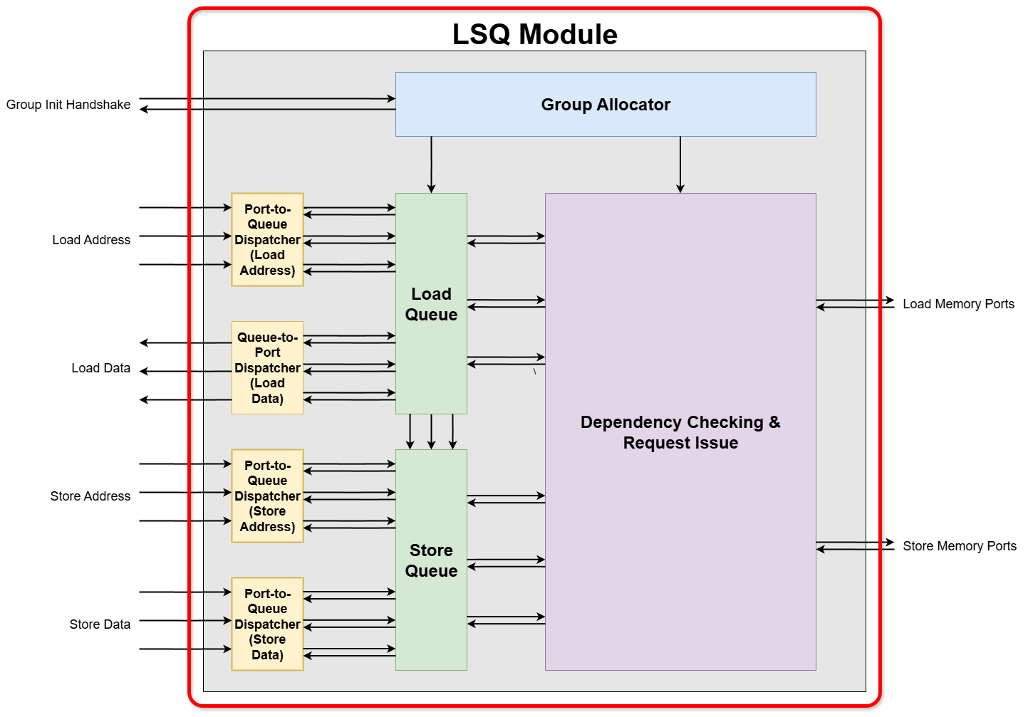
The LSQ is the system for managing all memory operations within the dataflow circuit. Its primary role is to accept out-of-order memory requests, track their dependencies, issue them to memory when safe, and return results in the correct order to the appropriate access ports. It also includes an any-to-any bypass network, which allows store data to be forwarded directly to subsequent loads to the same address without a memory round-trip.
The LSQ module acts as the master architect, instantiating the previously generated modules such as Port-to-Queue Dispatcher, Queue-to-Port Dispatcher, and Group Allocator modules. It wires them together with the load queue, the store queue, the dependency checking logic, and the requesting issue logic.
1.1. Configuration
The LSQ is configured through a JSON file that is passed to the Python generator. There are two categories of options:
- Required for Corretness:
These options must be set correctly to ensure programm correctness and that the LSQ interface matches what is expected by the compiler.
These options are set by the compiler using information it has about the circuit.
This includes:
- Number of groups
- Number of load and store ports in each group
- Relative order of loads and stores in each group
- Address bit width
- Data bit width
- …
- Optional Configuration:
These options can be used to tune performance, critical path, and/or resource usage of the LSQ.
They are currently fixed to default values, and no method to change them is exposed to users of Dynamatic.
This includes:
- Size of the load and store queues (default: both 16)
- Pipeline configuration (see Pipelining; default: all disabled)
- Bypass enable/disable (default: enabled)
All available options are described in configs.py.
2. LSQ Internal Blocks
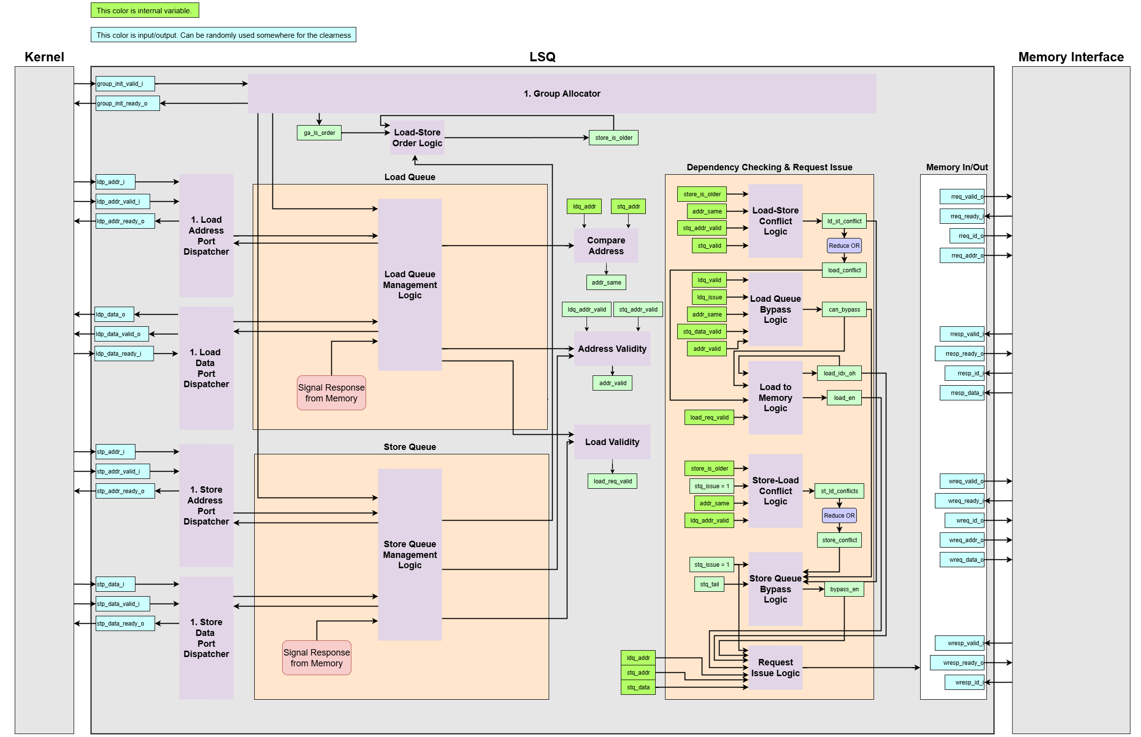
Let’s assume the following generic parameters for dimensionality:
N_GROUPS: The total number of groups.N_LDQ_ENTRIES: The total number of entries in the Load Queue.N_STQ_ENTRIES: The total number of entries in the Store Queue.LDQ_ADDR_WIDTH: The bit-width required to index an entry in the Load Queue (i.e.,ceil(log2(N_LDQ_ENTRIES))).STQ_ADDR_WIDTH: The bit-width required to index an entry in the Store Queue (i.e.,ceil(log2(N_STQ_ENTRIES))).LDP_ADDR_WIDTH: The bit-width required to index the port for a load.STP_ADDR_WIDTH: The bit-width required to index the port for a store.
Signal Naming and Dimensionality: This module is generated from a higher-level description (e.g., in Python), which results in a specific convention for signal naming in the final VHDL code. It’s important to understand this convention when interpreting the signal tables.
-
Generation Pattern: A signal that is conceptually an array in the source code is “unrolled” into multiple, distinct signals in the VHDL entity. The generated VHDL signals are indexed with a suffix, such as
ldp_addr_{p}_i, where{p}represents the port index. -
Placeholders: In the VHDL Signal Name column, the following placeholders are used:
{g}: Group index{lp}: Load port index{sp}: Store port index{lm}: Load memory channel index{sm}: Store memory channel index
-
Interpreting Diagrams: If a diagram or conceptual description uses a base name without an index (e.g.,
group_init_valid_i), it represents a collection of signals. The actual dimension is expanded based on the context:- Group-related signals (like
group_init_valid_i) are expanded by the number of groups (N_GROUPS). - Load queue-related signals (like
ldq_wen_o) are expanded by the number of load queue entries (N_LDQ_ENTRIES). - Store queue-related signals (like
stq_wen_o) are expanded by the number of store queue entries (N_STQ_ENTRIES).
- Group-related signals (like
2.1. Group Allocation Interface
These signals manage the handshake protocol for allocating groups of memory operations into the LSQ.
| Python Variable Name | VHDL Signal Name | Direction | Dimensionality | Description |
|---|---|---|---|---|
group_init_valid_i | group_init_valid_{g}_i | Input | std_logic | Valid signal from the kernel, indicating a request to allocate group {g}. |
group_init_ready_o | group_init_ready_{g}_o | Output | std_logic | Ready signal to the kernel, indicating the LSQ can accept a request for group {g}. |
2.2. Access Port Interface
This interface handles the flow of memory operation payloads (addresses and data) between the dataflow circuit’s access ports and the LSQ.
2.2.1. Load Address Dispatcher
Dispatches load addresses from the kernel to the load queue.
| Python Variable Name | VHDL Signal Name | Direction | Dimensionality | Description |
|---|---|---|---|---|
ldp_addr_i | ldp_addr_{lp}_i | Input | std_logic_vector(addrW-1:0) | The memory address for a load operation from load port {lp}. |
ldp_addr_valid_i | ldp_addr_valid_{lp}_i | Input | std_logic | Asserts that the payload on ldp_addr_{lp}_i is valid. |
ldp_addr_ready_o | ldp_addr_ready_{lp}_o | Output | std_logic | Asserts that the load queue is ready to accept an address from load port {lp}. |
2.2.1. Load Data Dispatcher
Returns data retrieved from memory back to the correct load port.
| Python Variable Name | VHDL Signal Name | Direction | Dimensionality | Description |
|---|---|---|---|---|
ldp_data_o | ldp_data_{lp}_o | Output | std_logic_vector(dataW-1:0) | The data payload being sent to load port {lp}. |
ldp_data_valid_o | ldp_data_valid_{lp}_o | Output | std_logic | Asserts that the payload on ldp_data_{lp}_o is valid. |
ldp_data_ready_i | ldp_data_ready_{lp}_i | Input | std_logic | Asserts that the kernel is ready to receive data on load port {lp}. |
2.2.3. Store Address Dispatcher
Dispatches store addresses from the kernel to the LSQ.
| Python Variable Name | VHDL Signal Name | Direction | Dimensionality | Description |
|---|---|---|---|---|
stp_addr_i | stp_addr_{sp}_i | Input | std_logic_vector(addrW-1:0) | The memory address for a store operation from store port {sp}. |
stp_addr_valid_i | stp_addr_valid_{sp}_i | Input | std_logic | Asserts that the payload on stp_addr_{sp}_i is valid. |
stp_addr_ready_o | stp_addr_ready_{sp}_o | Output | std_logic | Asserts that the store queue is ready to accept an address from store port {sp}. |
2.2.4. Store Data Dispatcher
Dispatches data to be stored from the kernel to the LSQ.
| Python Variable Name | VHDL Signal Name | Direction | Dimensionality | Description |
|---|---|---|---|---|
stp_data_i | stp_data_{sp}_i | Input | std_logic_vector(dataW-1:0) | The data payload to be stored from store port {sp}. |
stp_data_valid_i | stp_data_valid_{sp}_i | Input | std_logic | Asserts that the payload on stp_data_{sp}_i is valid. |
stp_data_ready_o | stp_data_ready_{sp}_o | Output | std_logic | Asserts that the store queue is ready to accept data from store port {sp}. |
2.3. Memory Interface
These signals form the connection between the LSQ and the main memory system.
Read Channel
2.3.1. Read Request (LSQ to Memory)
Used by the LSQ to issue load operations to memory.
| Python Variable Name | VHDL Signal Name | Direction | Dimensionality | Description |
|---|---|---|---|---|
rreq_valid_o | rreq_valid_{lm}_o | Output | std_logic | Valid signal indicating the LSQ is issuing a read request on channel {lm}. |
rreq_ready_i | rreq_ready_{lm}_i | Input | std_logic | Ready signal from memory, indicating it can accept a read request on channel {lm}. |
rreq_id_o | rreq_id_{lm}_o | Output | std_logic_vector(idW-1:0) | An ID for the read request, used to match the response. |
rreq_addr_o | rreq_addr_{lm}_o | Output | std_logic_vector(addrW-1:0) | The memory address to be read. |
2.3.2. Read Response (Memory to LSQ)
Used by memory to return data for a previously issued read request.
| Python Variable Name | VHDL Signal Name | Direction | Dimensionality | Description |
|---|---|---|---|---|
rresp_valid_i | rresp_valid_{lm}_i | Input | std_logic | Valid signal from memory, indicating a read response is available on channel {lm}. |
rresp_ready_o | rresp_ready_{lm}_o | Output | std_logic | Ready signal to memory, indicating the LSQ can accept the read response. |
rresp_id_i | rresp_id_{lm}_i | Input | std_logic_vector(idW-1:0) | The ID of the read response, matching a previous rreq_id_o. |
rresp_data_i | rresp_data_{lm}_i | Input | std_logic_vector(dataW-1:0) | The data returned from memory. |
Write Channel
2.3.3. Write Request (LSQ to Memory)
Used by the LSQ to issue store operations to memory.
| Python Variable Name | VHDL Signal Name | Direction | Dimensionality | Description |
|---|---|---|---|---|
wreq_valid_o | wreq_valid_{sm}_o | Output | std_logic | Valid signal indicating the LSQ is issuing a write request on channel {sm}. |
wreq_ready_i | wreq_ready_{sm}_i | Input | std_logic | Ready signal from memory, indicating it can accept a write request on channel {sm}. |
wreq_id_o | wreq_id_{sm}_o | Output | std_logic_vector(idW-1:0) | An ID for the write request. |
wreq_addr_o | wreq_addr_{sm}_o | Output | std_logic_vector(addrW-1:0) | The memory address to write to. |
wreq_data_o | wreq_data_{sm}_o | Output | std_logic_vector(dataW-1:0) | The data to be written to memory. |
2.3.4. Write Response (Memory to LSQ)
Used by memory to signal the completion of a write operation.
| Python Variable Name | VHDL Signal Name | Direction | Dimensionality | Description |
|---|---|---|---|---|
wresp_valid_i | wresp_valid_{sm}_i | Input | std_logic | Valid signal from memory, indicating a write has completed on channel {sm}. |
wresp_ready_o | wresp_ready_{sm}_o | Output | std_logic | Ready signal to memory, indicating the LSQ can accept the write response. |
wresp_id_i | wresp_id_{sm}_i | Input | std_logic_vector(idW-1:0) | The ID of the completed write. |
The LSQ has the following responsibilities:
- Sub-Module Instantiation
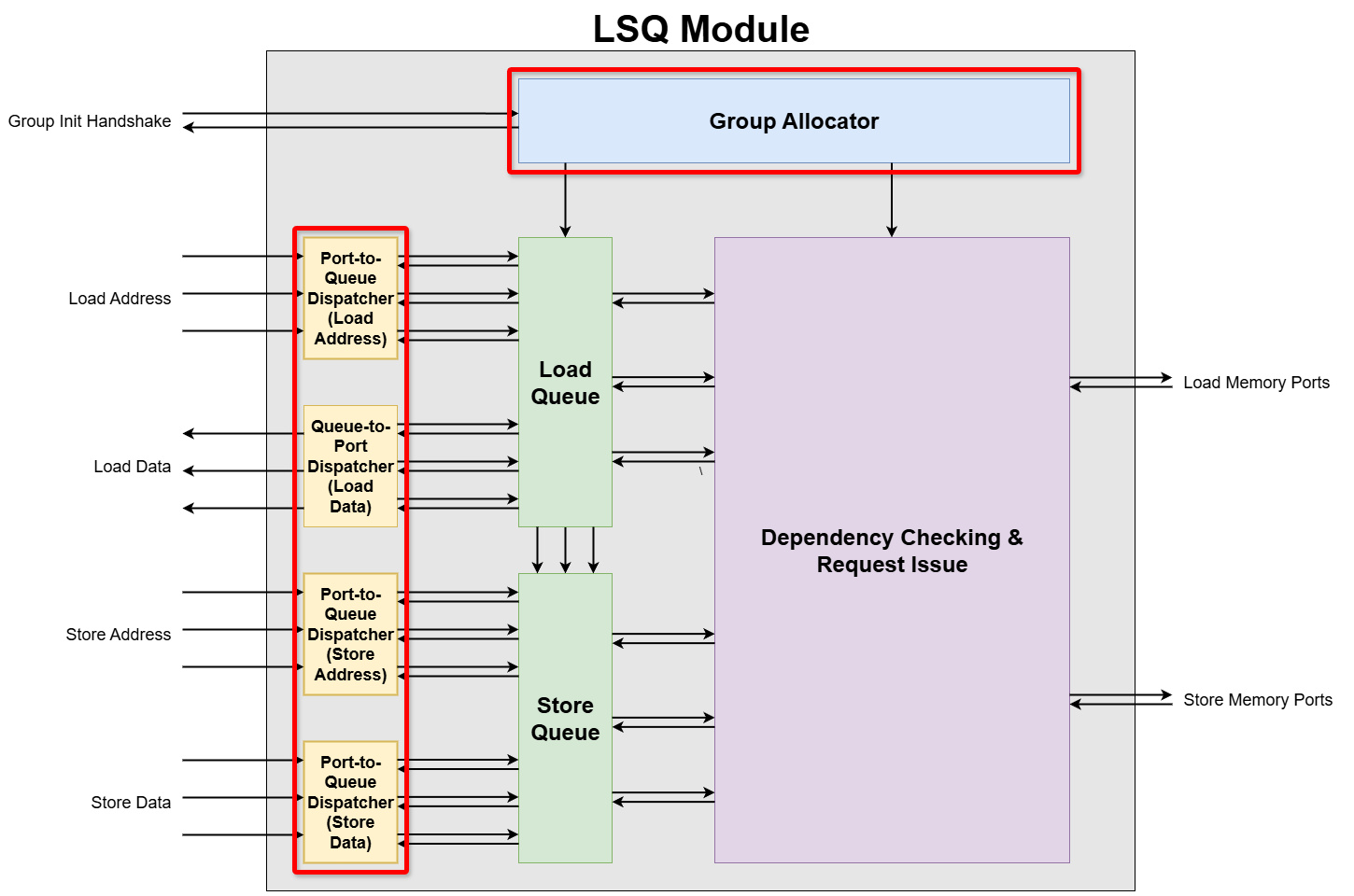 The primary responsibility of the top-level LSQ module is to function as an integrator. It instantitates several specialized sub-modules and connects them with the load queue, the store queue, dependency checking logic, and requesting issue logic to create the complete memory management system.
- Group Allocator: This module is responsible for managing entry allocation for the LSQ. It performs the initial handshake to reserve entries for an entire group of loads and stores, providing the necessary ordering information that would otherwise be missing in a dataflow circuit.
- Port-to-Queue (PTQ) Dispatcher: This module is responsible for routing incoming payloads, such as addresses and data, from the dataflow circuit’s external access ports to the correct entries within the load queue and the store queue. The LSQ instantiates three distinct PTQ dispatchers:
- Load Address Port Dispatcher: For routing load addresses.
- Store Address Port Dispatcher: For routing store addresses.
- Store Data Port Dispatcher: For routing store data.
- Queue-to-Port (QTP) Dispatcher: This module is the counterparts to the PTQ dispatchers. It takes payloads from the queue entries and route them back to the correct external access ports. The LSQ instantiates the following QTP dispatchers:
- Load Data Port Dispatcher: Sends loaded data back to the circuit.
- (Optionally) Store Backward Port Dispatcher: It is used to send store completion acknowledgements back to the circuit if the
stRespconfiguration is enabled.
-
Load Queue Management Logic
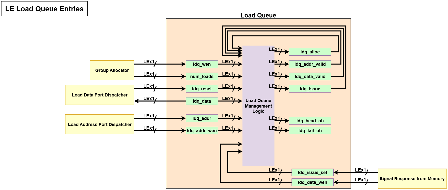 This block can be divided into three sub-block: Load Queue Entry Allocation Logic, Load Queue Pointer Logic, and Load Queue Content State Logic.
2.1. Load Queue Entry Allocation Logic
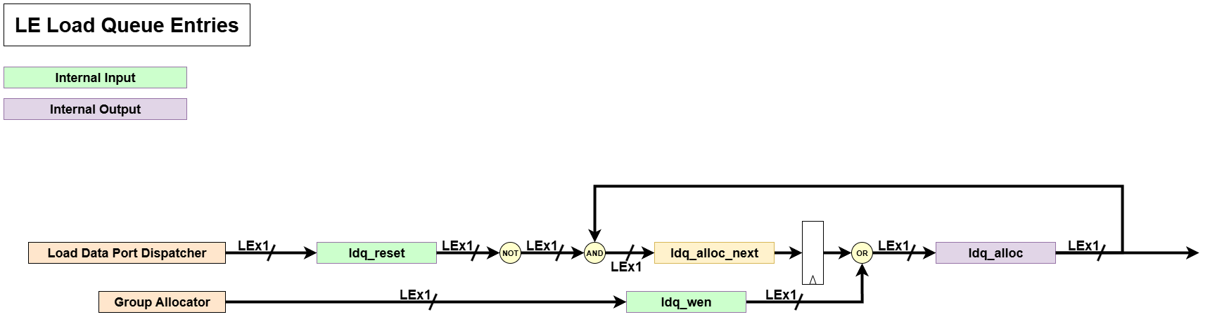 This block checks whether each queue entry is allocated or deallocated.
- Input:
ldq_wen: A signal from the Group Allocator that goes high to activate the queue entry when a new load group is being allocated.ldq_reset: A signal from the Load Data Port Dispatcher that goes high to deactivate (reset) the entry after its load operation is complete and the data has been sent to the kernel.ldq_alloc(current state): The current allocation status from the register’s output, which is fed back as an input to the logic.
- Processing:
- The
ldq_resetsignal is inverted by aNOTgate. The result represents the “do not reset” condition. - This inverted signal is then combined with the current
ldq_allocstate using anANDgate. The result of this operation (labeledldq_alloc_nextin concept) is ‘1’ only if “the entry is currently allocated AND it is not being reset,” indicating that the allocation should be maintained. - The output of the
ANDgate is then combined with theldq_wensignal using anORgate. This final logic determines that the entry will be in an allocated state (‘1’) during the next clock cycle if either of two conditions is met:- A new allocation is requested (
ldq_wen= ‘1’). - It was already allocated and no reset was requested (
ldq_alloc= ‘1’ ANDldq_reset= ‘0’).
- A new allocation is requested (
- This logic is equivalent to the expression
next_state <= ldq_wen OR (ldq_alloc AND NOT ldq_reset).
- The
- Output:
ldq_alloc(next state): The updated allocation status of the load queue entry for the subsequent clock cycle. This signal is used by other logic within the LSQ to determine if the entry is active.
2.2. Load Queue Pointer Logic
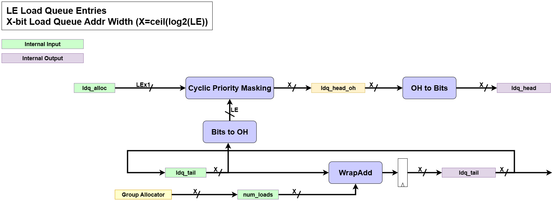 This block is dedicated to calculating the next positions of the head and tail pointers of the circular queue.
-
Input:
num_loads: The number of new entries being allocated. From the Group Allocator.ldq_tail(current state): The current tail pointer value.ldq_alloc: The up-to-date allocation status vector for all entries, which is the output of the Entry State Logic.
-
Processing:
- Tail Pointer Update: When a new group is allocated, it advances the
ldq_tailpointer by thenum_loadsamount, usingWrapAddto handle the circular nature of the queue. - Head Pointer Update: It determines the next
ldq_headby usingCyclicPriorityMaskingon theldq_allocvector. This efficiently finds the oldest, active entry, which becomes the new head.
- Tail Pointer Update: When a new group is allocated, it advances the
-
Output:
ldq_head(next state): The updated head pointer of the queue.ldq_tail(next state): The updated tail pointer of the queue.
2.3. Load Queue Content State Logic
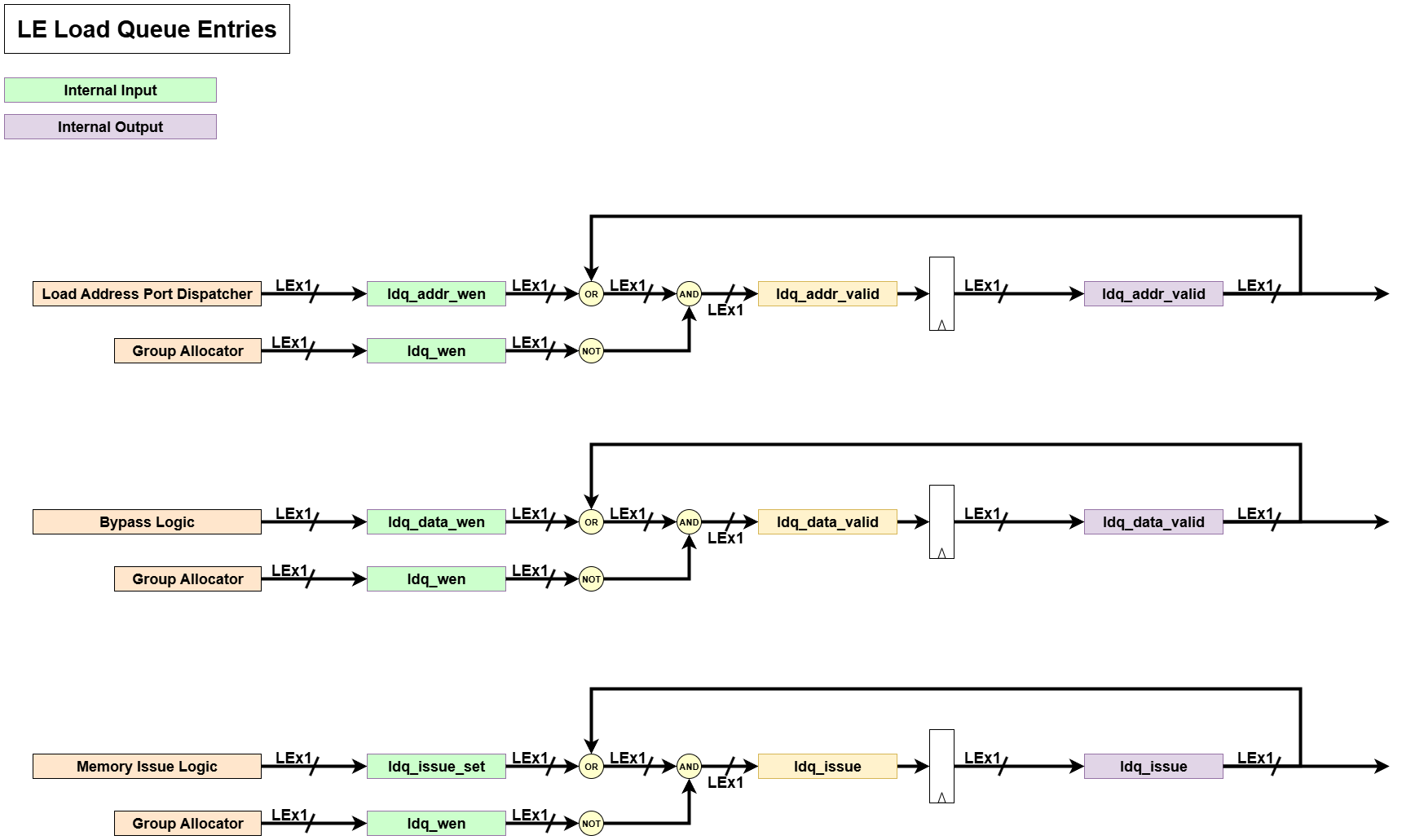
This logic manages the validity status of the various payloads and the issue status within an allocated entry. All signals in this block share a similar structure.
-
Input:
- Set Signals:
ldq_addr_wen: From the Load Address Port Dispatcher, setsldq_addr_validto true.ldq_data_wen: From the Bypass Logic or memory interface, setsldq_data_validto true.ldq_issue_set: From the Dependency Checking & Issue Logic, setsldq_issueto true.
- Common Reset Signal:
ldq_wen: From the Group Allocator. It acts as a synchronous reset for all these status bits, clearing them to ‘0’ when a new operation is allocated to the entry.
- Current State Signals:
ldq_addr_valid(curr state): Current status indicating if the entry holds a valid address.ldq_data_valid(curr state): Current status indicating if the entry holds valid data.ldq_issue(curr state): Current status indicating if the load request has been satisfied.
- Set Signals:
-
Processing:
- All three signals (
ldq_addr_valid,ldq_data_valid,ldq_issue) follow the same Set-Reset flip-flop logic pattern, whereldq_wenhas reset priority. - A status bit is set if its corresponding “set” signal (e.g.,
ldq_addr_wen) is high. If not being set, it holds its value. - However, if
ldq_wenis high for an entry, all three status bits for that entry are unconditionally cleared to ‘0’ on the next clock cycle. - The logic is equivalent to these expressions:
ldq_addr_valid_next <= (ldq_addr_wen OR ldq_addr_valid) AND (NOT ldq_wen)ldq_data_valid_next <= (ldq_data_wen OR ldq_data_valid) AND (NOT ldq_wen)ldq_issue_next <= (ldq_issue_set OR ldq_issue) AND (NOT ldq_wen)
- All three signals (
-
Output:
ldq_addr_valid(next state): Updated status indicating if the entry holds a valid address.ldq_data_valid(next state): Updated status indicating if the entry holds valid data.ldq_issue(next state): Updated status indicating if the load request has been satisfied.
- Input:
-
Store Queue Management Logic
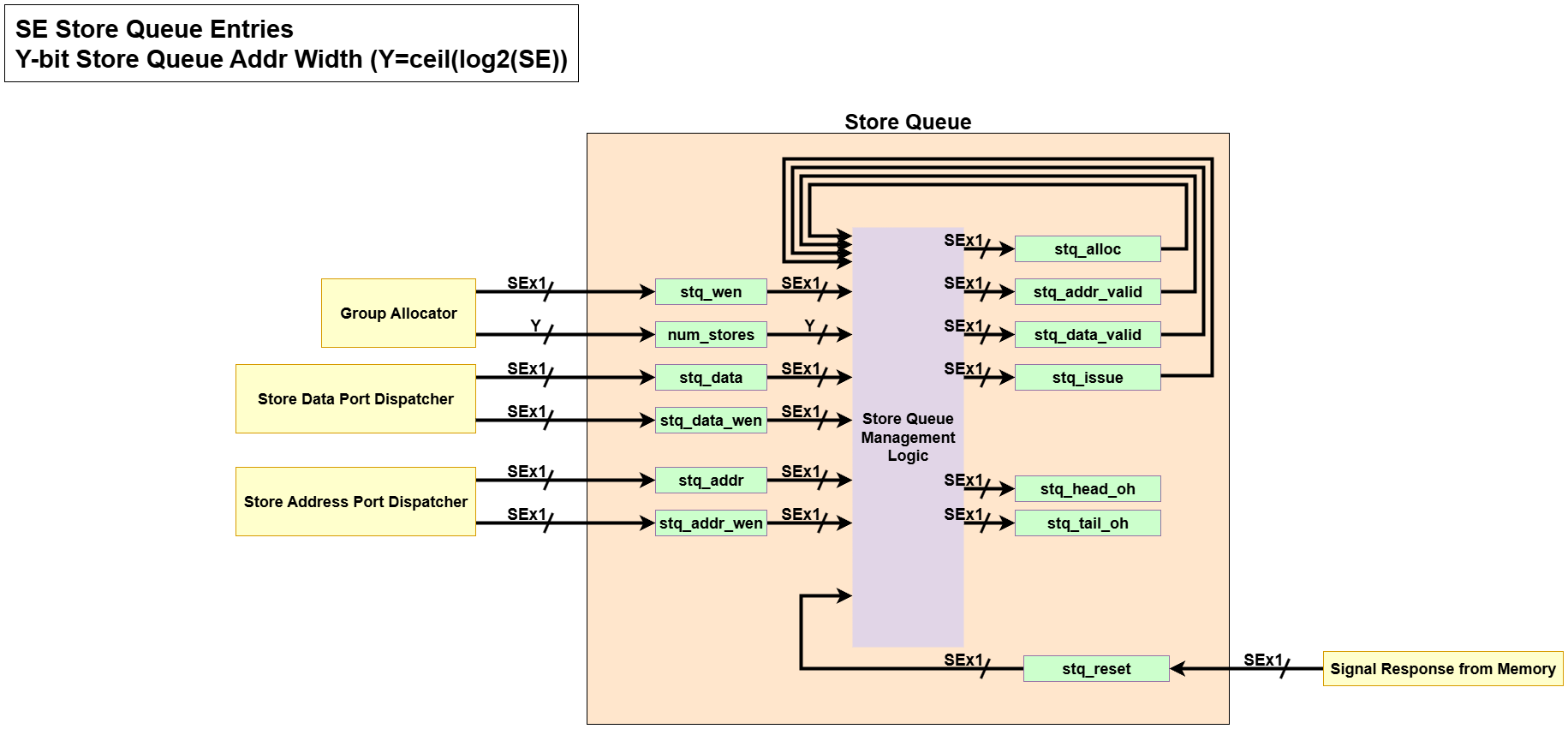
This block can be divided into three sub-block: Store Queue Entry Allocation Logic, Store Queue Pointer Logic, and Store Queue Content State Logic.3.1. Store Queue Entry Allocation Logic (
stq_alloc)
This logic manages the allocation status for each entry in the Store Queue (STQ), indicating whether it is active.-
Input:
stq_wen: The write-enable signal from the Group Allocator. When high, it signifies that this entry is being allocated to a new store operation.stq_reset: The reset signal, which can be triggered by a write response (wresp_valid_i) or by a store backward dispatch (qtp_dispatcher_stb). When high, it deallocates the entry.stq_alloc(current state): The current allocation status from the register’s output, fed back as an input.
-
Processing:
- The logic follows the same Set-Reset principle as the load queue.
- The entry becomes allocated (
'1') if a new store is being written to it (stq_wenis high). - It remains allocated if it was already allocated and is not being reset.
- The logic is equivalent to the expression:
stq_alloc_next <= stq_wen OR (stq_alloc AND NOT stq_reset).
-
Output:
stq_alloc(next state): The updated allocation status vector. This signal is used to identify which store entries are currently active.
3.2. Store Queue Pointer Logic
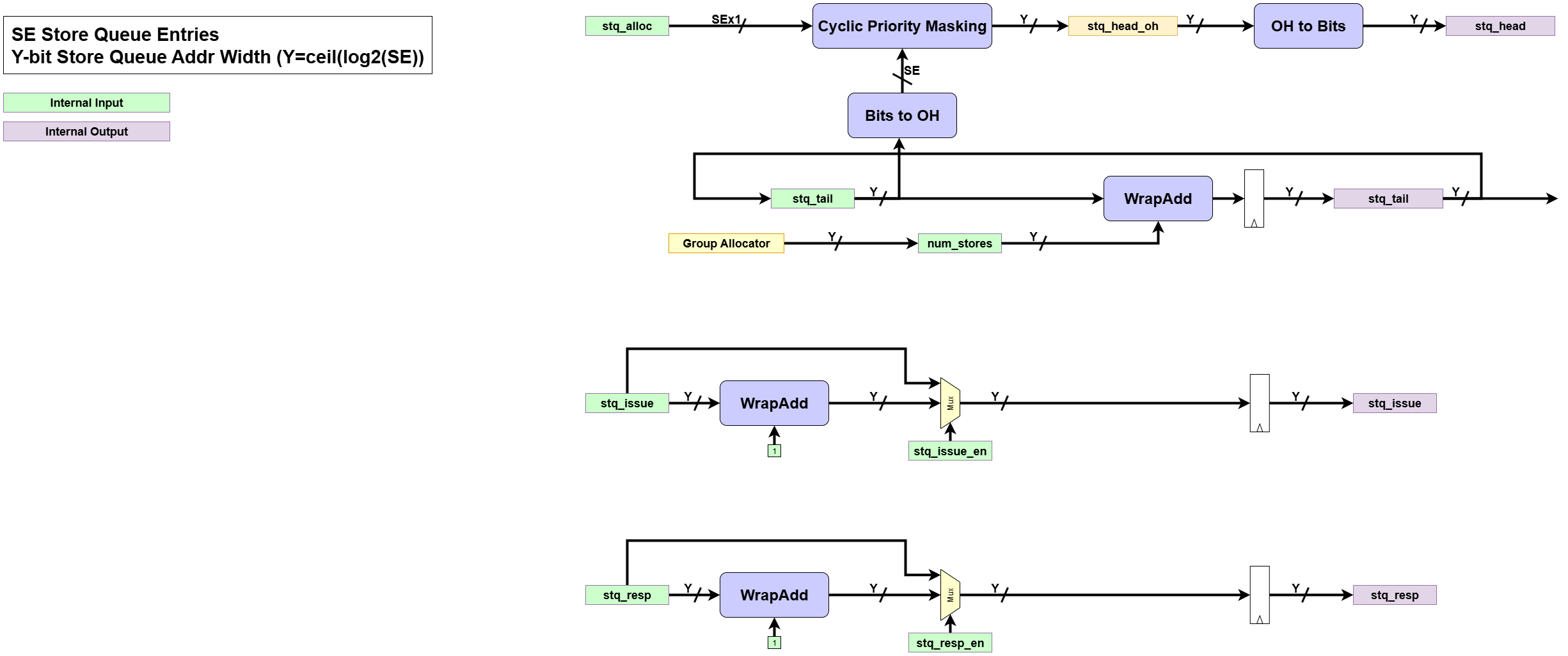
This block manages the four distinct pointers associated with the Store Queue:head,tail,issue, andresp.-
Input:
num_stores: The number of new entries being allocated. From the Group Allocator.stq_tail,stq_head,stq_issue,stq_resp(current states): The current values of the pointers.stq_alloc: The up-to-date allocation status vector for all entries.stq_issue_en: An enable signal from the Request Issue Logic that allows thestq_issuepointer to advance.stq_resp_en: An enable signal, typically tied towresp_valid_i, that allows thestq_resppointer to advance.
-
Processing:
- Tail Pointer Update: The
stq_tailpointer is advanced bynum_storesusingWrapAddupon new group allocation. - Head Pointer Update: The
stq_headpointer advances to the next oldest active entry. Its logic can depend on the configuration (e.g., advancing on a write response or usingCyclicPriorityMasking). - Issue Pointer Update: The
stq_issuepointer, which tracks the next store to be considered for memory issue, is incremented by one whenstq_issue_enis high. - Response Pointer Update: The
stq_resppointer, which tracks completed write operations from memory, is incremented by one whenstq_resp_enis high.
- Tail Pointer Update: The
-
Output:
stq_head,stq_tail,stq_issue,stq_resp(next states): The updated pointer values for the next cycle.
3.3. Store Queue Content State Logic
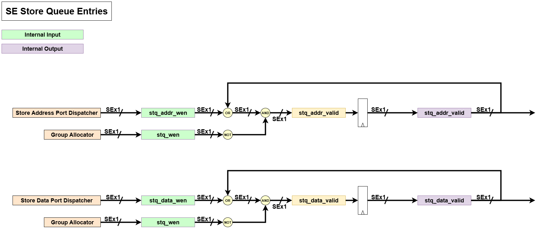
This logic manages the validity of the address and data payloads, as well as the execution status, within an allocated store entry.-
Input:
- Set Signals:
stq_addr_wen: From the Store Address Port Dispatcher, setsstq_addr_validto true.stq_data_wen: From the Store Data Port Dispatcher, setsstq_data_validto true.stq_exec_set: (Optional, ifstResp=True) From the memory interface, setsstq_execto true upon write completion.
- Common Reset Signal:
stq_wen: From the Group Allocator. It acts as a synchronous reset, clearing these status bits when a new operation is allocated.
- Current State Signals:
stq_addr_valid,stq_data_valid,stq_exec: The current state of each register, fed back as an input.
- Set Signals:
-
Processing:
- All three signals (
stq_addr_valid,stq_data_valid,stq_exec) follow the same Set-Reset logic pattern, wherestq_wenhas reset priority. - A status bit is set if its corresponding “set” signal (e.g.,
stq_addr_wen) is high. If not being set, it holds its value. - However, if
stq_wenis high for an entry, all three status bits are unconditionally cleared to ‘0’. - The logic is equivalent to these expressions:
stq_addr_valid_next <= (stq_addr_wen OR stq_addr_valid) AND (NOT stq_wen)stq_data_valid_next <= (stq_data_wen OR stq_data_valid) AND (NOT stq_wen)stq_exec_next <= (stq_exec_set OR stq_exec) AND (NOT stq_wen)
- All three signals (
-
Output:
stq_addr_valid(next state): Updated status indicating if the entry holds a valid store address.stq_data_valid(next state): Updated status indicating if the entry holds valid store data.stq_exec(next state): (Optional) Updated status indicating if the store has been executed by memory.
-
- Load-Store Order Matrix Logic (
store_is_older)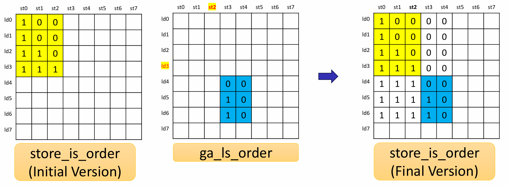 This logic maintains a 2D register matrix that captures the relative program order between every load and store in the queues. Its primary purpose is to provide a static record of dependencies for the conflict-checking logic.
-
Input:
ldq_wen: The write-enable signal from the Group Allocator. Whenldq_wen[i]is high, it triggers an update for rowiof the matrix.stq_alloc: The allocation status vector from the Store Queue Management Logic. This is used to identify any stores that were already in the queue before the new load was allocated.ga_ls_order: A matrix from the Group Allocator that specifies the ordering within the newly allocated group.ga_ls_order[i][j]is ‘1’ if storejis older than loadiin the same group.stq_reset: The reset signal for store entries. Whenstq_reset[j]is high, it clears columnjof the matrix, removing the completed store as a dependency.store_is_older(current state): The current state of the matrix, fed back as an input.
-
Processing:
- The logic for
store_is_older[i][j]determines if storejshould be considered older than loadi. This state is set once when loadiis allocated and then only changes if storejis deallocated. - On Load Allocation (
ldq_wen[i]is high): The entire rowiof the matrix is updated. For each storej, the bitstore_is_older[i][j]is set to ‘1’ if the store is not being reset (NOT stq_reset[j]) AND one of the following is true:- The store
jwas already active in the queue when loadiarrived (stq_alloc[j]is ‘1’). - The store
jis part of the same new group as loadiand is explicitly defined as older (ga_ls_order[i][j]is ‘1’).
- The store
- On Store Deallocation (
stq_reset[j]is high): The logic clears the entire columnjto ’0’s. This ensures that a completed store is no longer considered a dependency for any active loads. - Hold State: If no new load is being allocated to row
i, the row maintains its existing values, except for any bits that are cleared due to a store deallocation.
- The logic for
-
Output:
store_is_older(next state): The updated dependency matrix. This matrix is a critical input for both the Load-Store Conflict Logic and the Store-Load Conflict Logic. A ‘1’ atstore_is_older[i][j]essentially means “loadimust respect storej.”
- Compare Address Logic (
addr_same)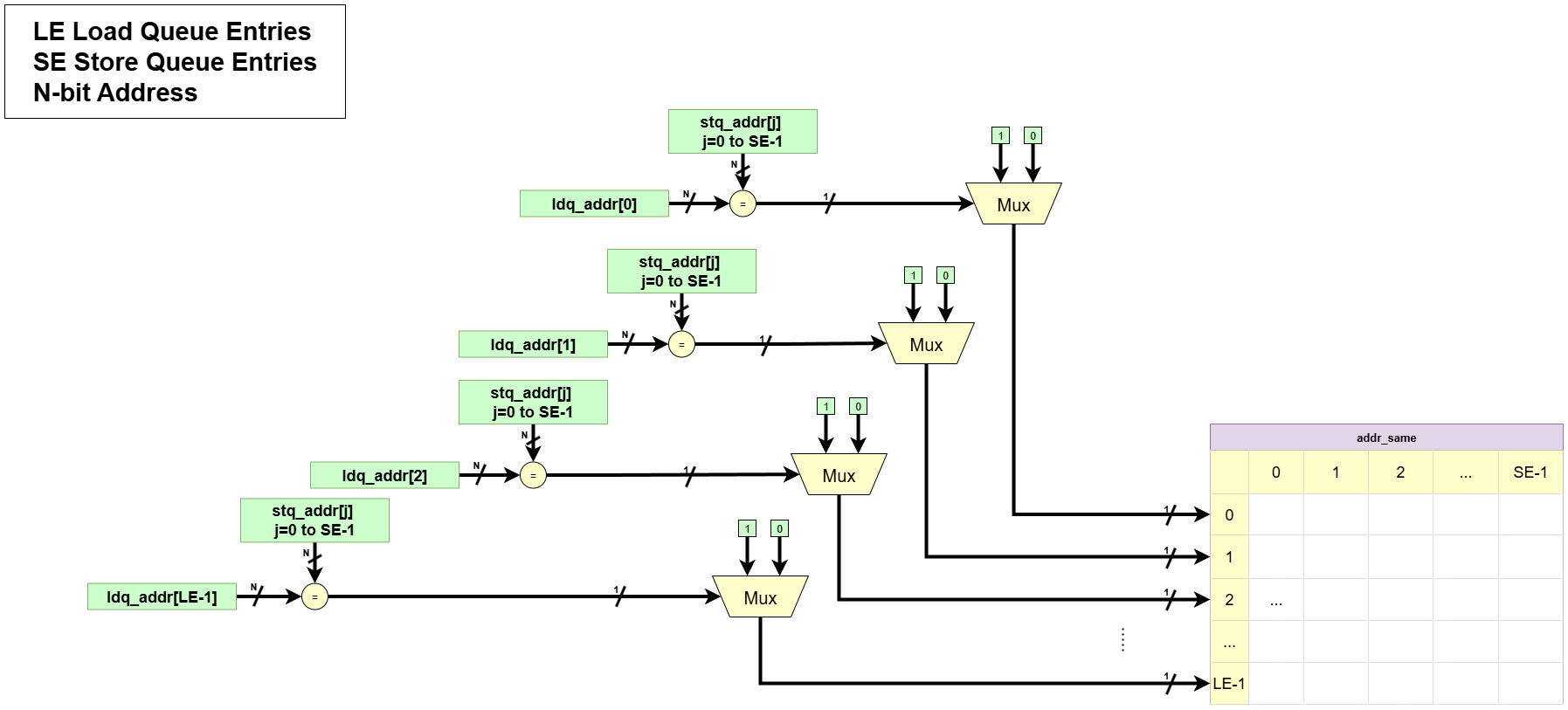 This combinational logic block performs a direct comparison between every load address and every store address in the queues.
-
Input:
ldq_addr: The array of all addresses stored in the Load Queue.stq_addr: The array of all addresses stored in the Store Queue.
-
Processing:
- For every possible pair of a load
iand a storej, it performs a direct equality comparison:ldq_addr[i] == stq_addr[j].
- For every possible pair of a load
-
Output:
addr_same: A 2D matrix where the bit at[i, j]is ‘1’ if the addresses of loadiand storejare identical. This matrix is a fundamental input for both the conflict and bypass logic to detect potential address hazards.
- Address Validity Logic (
addr_valid)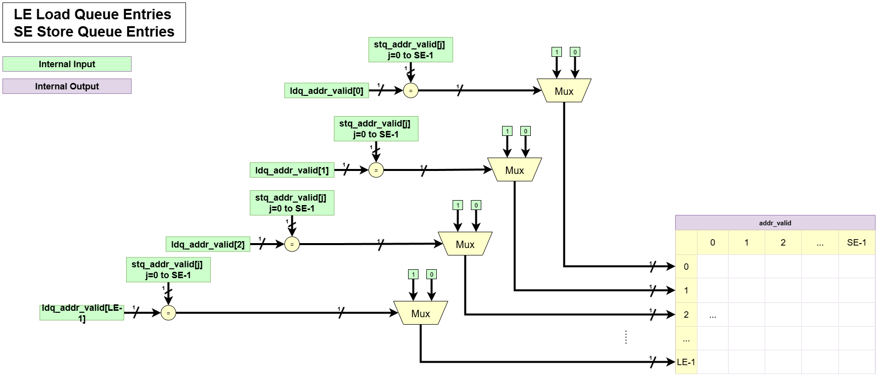 This logic checks whether both operations in a given load-store pair have received their addresses, making them eligible for a meaningful address comparison.
-
Input:
ldq_addr_valid: A vector indicating which LDQ entries have a valid address.stq_addr_valid: A vector indicating which STQ entries have a valid address.
-
Processing:
- For every possible pair of a load
iand a storej, it performs a logical AND operation:ldq_addr_valid[i] AND stq_addr_valid[j].
- For every possible pair of a load
-
Output:
addr_valid: A 2D matrix where the bit at[i, j]is ‘1’ only if both loadiand storejhave valid addresses. This is used to qualify bypass conditions, ensuring a bypass is only considered when both addresses are known.
- Load Request Validity Logic (
load_req_valid)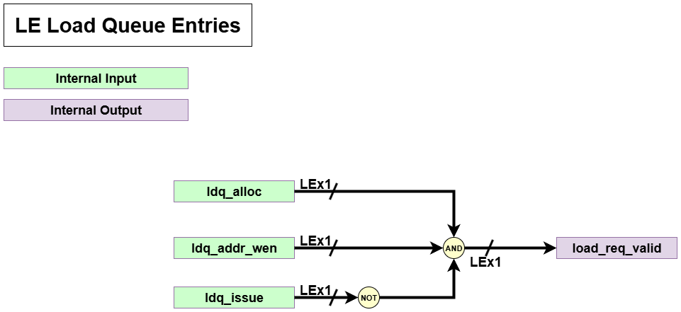 This logic block generates a list of loads that are ready to be evaluated by the dependency checker. It filters out loads that are not yet active or have already been completed.
-
Input:
ldq_alloc: The vector indicating which load queue entries are currently allocated and active.ldq_issue: The vector indicating which load requests have already been satisfied (either by being sent to memory or through a bypass).ldq_addr_valid: The vector indicating which active loads have received their address payload.
-
Processing:
- For each load entry
i, it performs a logical AND across three conditions to determine if it’s a valid candidate for issue:- The entry must be allocated (
ldq_alloc[i]). - The address must be valid (
ldq_addr_valid[i]). - The request must not have been previously issued (
NOT ldq_issue[i]).
- The entry must be allocated (
- The complete expression is
ldq_alloc[i] AND ldq_addr_valid[i] AND (NOT ldq_issue[i]).
- For each load entry
-
Output:
load_req_valid: A vector where a ‘1’ at indexisignifies that loadiis an active request that is ready to be checked for dependencies. This vector serves as the primary input pool for the Load to Memory Logic.
- Load-Store Conflict Logic
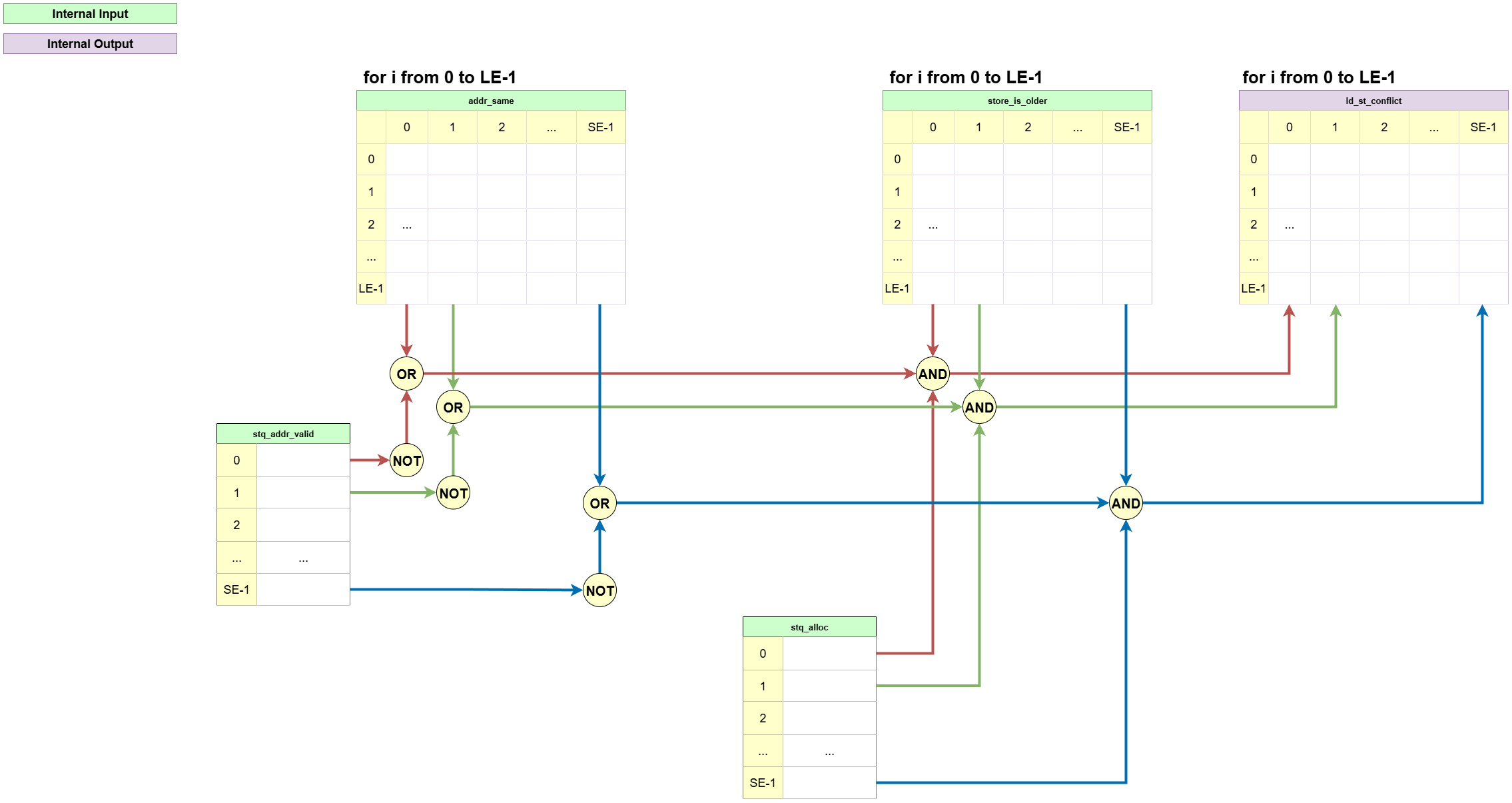 This is the primary logic for ensuring load safety. It checks every active load against every active store to see if the load must wait for the store to complete.
-
Input:
stq_alloc: A vector indicating which store queue entries are active.store_completed: A vector indicating whether a store has already received its response from memory.store_is_older: The 2D matrix establishing the program order between loads and stores.addr_same: The 2D matrix indicating which load-store pairs have identical addresses.stq_addr_valid: A vector indicating which stores have a valid address.
-
Processing:
- It calculates the
ld_st_conflictmatrix. A conflict atld_st_conflict[i][j]is asserted (‘1’) if all of the following are true:- The store
jis allocated (stq_alloc[j]). - The store
jhas not completed (NOT store_completed[j]). - The store
jis older than the loadi(store_is_older[i][j]). - A potential address hazard exists, which means either:
- Their addresses are identical (
addr_same[i][j]). - OR the store’s address is not yet known (
NOT stq_addr_valid[j]).
- Their addresses are identical (
- The store
- It calculates the
-
Output:
ld_st_conflict: A 2D matrix where a ‘1’ at[i, j]signifies that loadihas a dependency on storejand must not be issued to memory ifjis also pending.
- Load Queue Bypass Logic (Determining Bypass Potential)
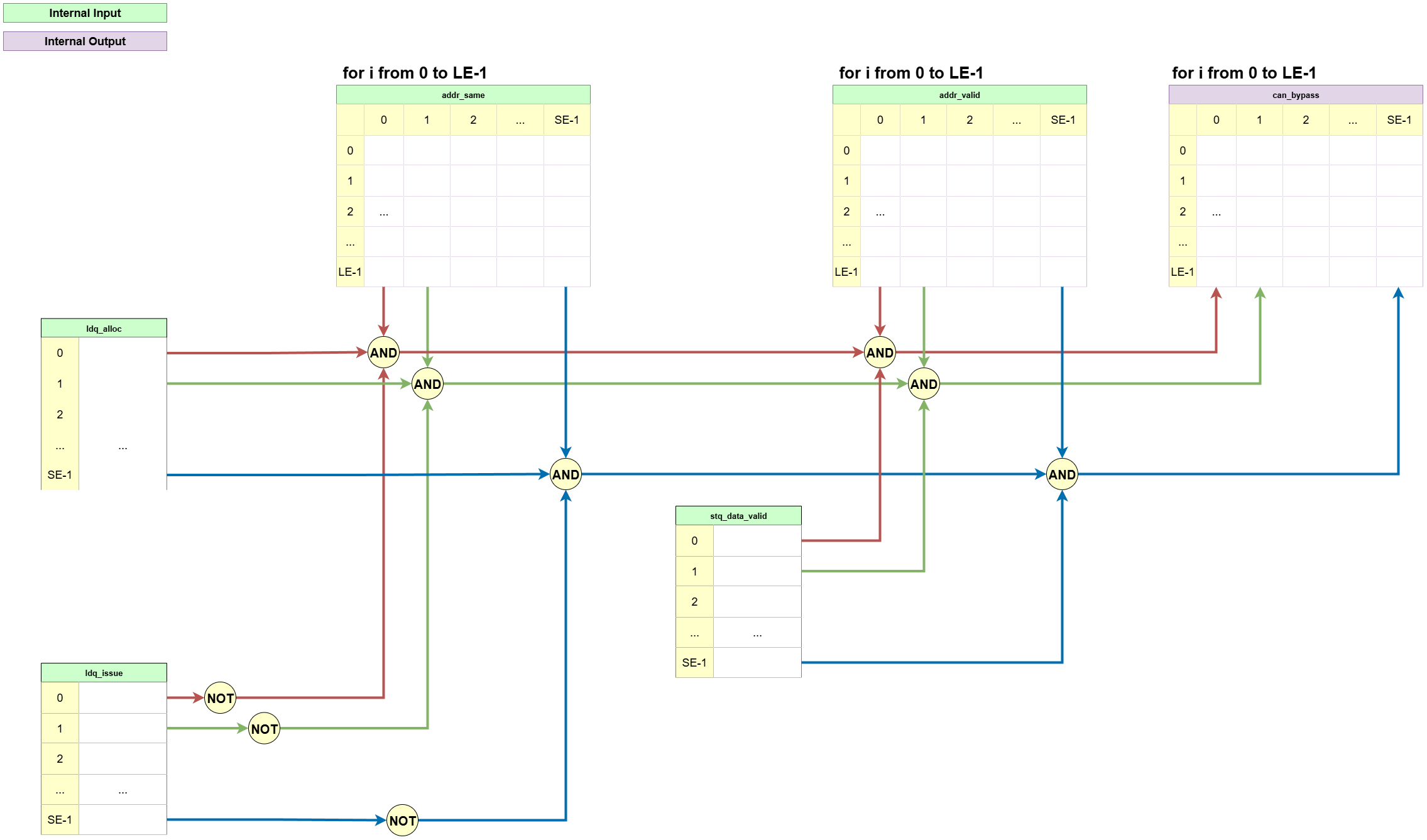 This block determines for which load-store pairs a bypass (store-to-load forwarding) is potentially possible.
Note: The bypass logic can be disabled by setting the config parameter
bypasstoFalse. In that case,bypass_enis tied to constant zero, which enables the synthesizer to optimize out the entire bypass logic (including thecan_bypassmatrix). This can significantly lower the LSQ’s resource cost (e.g., by around 50% forhistogramwith 16-entry load and store queues).
-
Input:
ldq_alloc: A vector indicating which load queue entries are active.ldq_issue: A vector indicating which loads have already been satisfied.stq_data_valid: A vector indicating which store entries have valid data ready for forwarding.addr_same: The address equality matrix.addr_valid: The matrix indicating pairs with valid addresses.
-
Processing:
- It calculates the
can_bypassmatrix. A bitcan_bypass[i][j]is asserted if all conditions for a potential bypass are met:- The load
iis active (ldq_alloc[i]). - The load
ihas not been issued yet (NOT ldq_issue[i]). - The store
jhas valid data (stq_data_valid[j]). - Both the load and store have valid and identical addresses (
addr_valid[i][j]andaddr_same[i][j]).
- The load
- It calculates the
-
Output:
can_bypass: A 2D matrix indicating every load-store pair where a bypass is theoretically possible. This matrix is used as an input to the logic that makes the final bypass decision.
- Load to Memory Logic
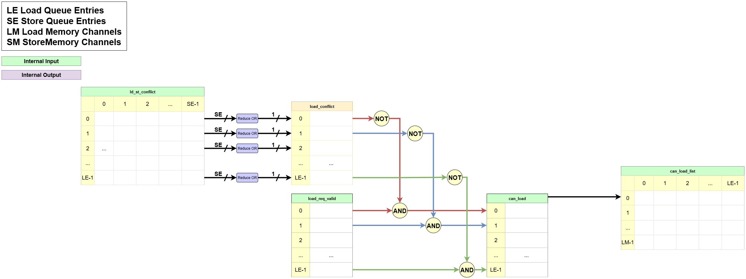 This logic block makes the final decision on which loads are safe to issue to the memory interface.
-
Input:
ld_st_conflict: The dependency matrix from the Load-Store Conflict Logic.load_req_valid: A vector indicating which loads are active and ready to be checked.ldq_head_oh: The one-hot head pointer of the load queue, used to prioritize the oldest requests.
-
Processing:
- First, it OR-reduces each row of the
ld_st_conflictmatrix to create a singleload_conflictbit for each load. - It then creates a list of issue candidates,
can_load, by selecting requests fromload_req_validthat are not blocked (NOT load_conflict). - Finally, it uses
CyclicPriorityMaskingon thecan_loadlist to arbitrate and select the oldest, highest-priority load(s) for the available memory read channel(s).
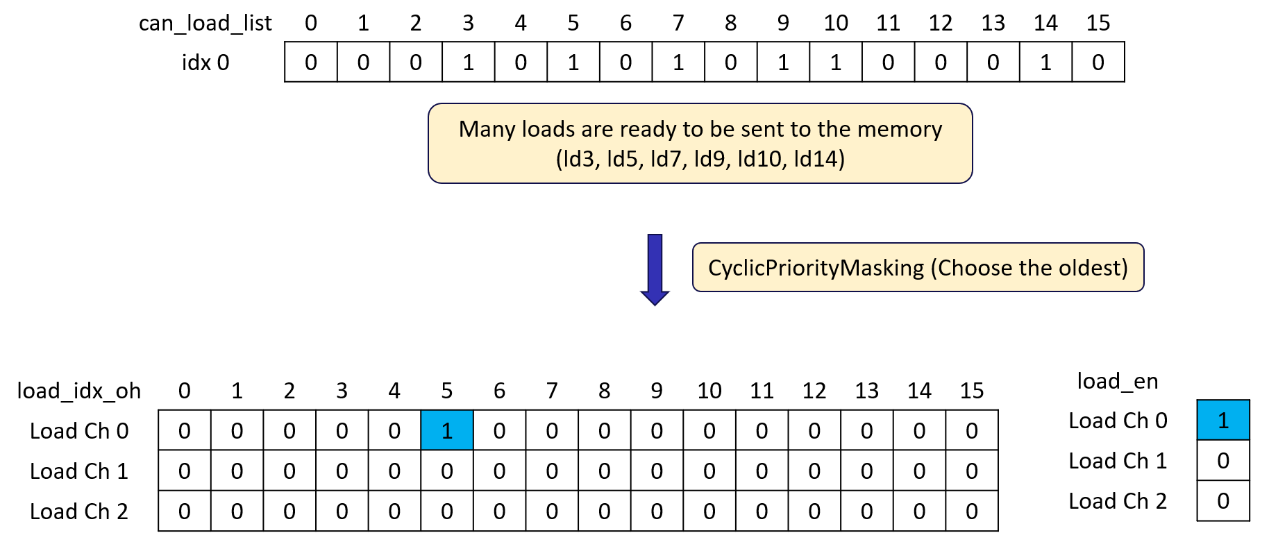
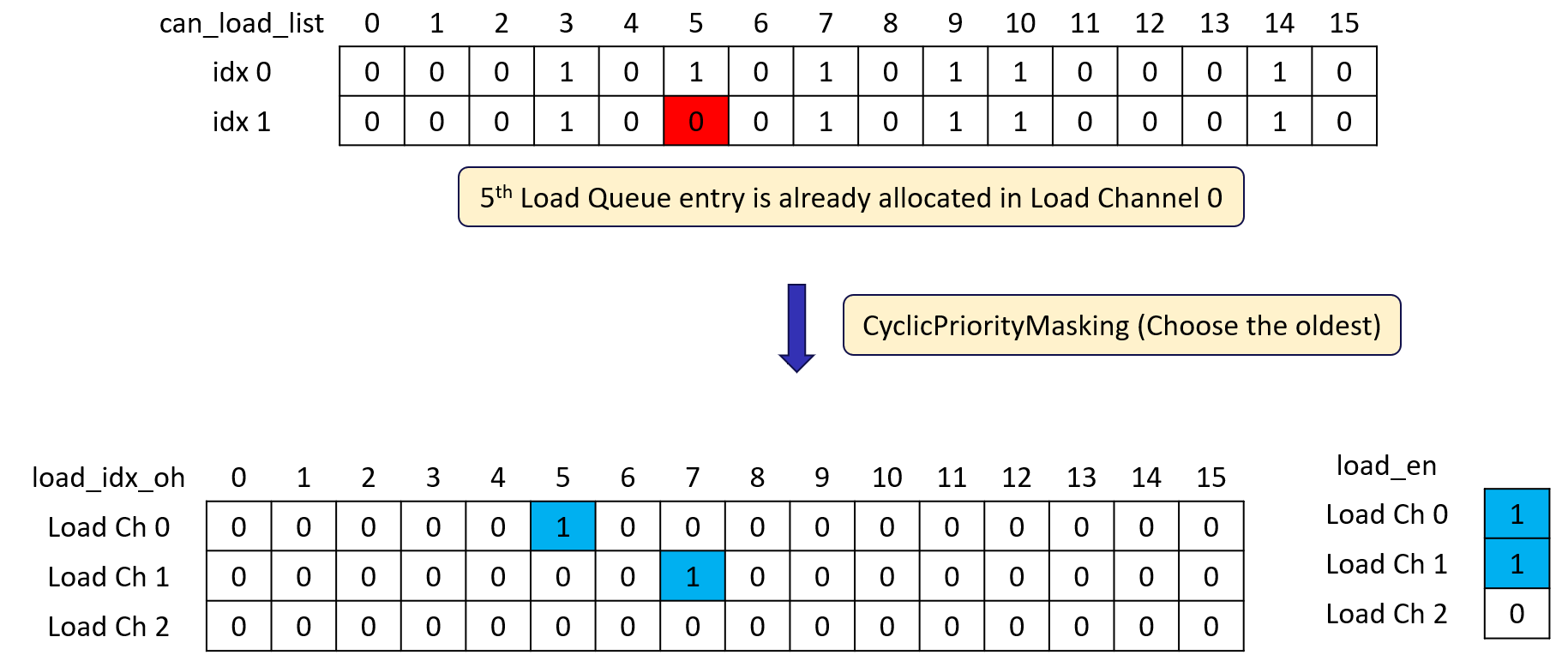
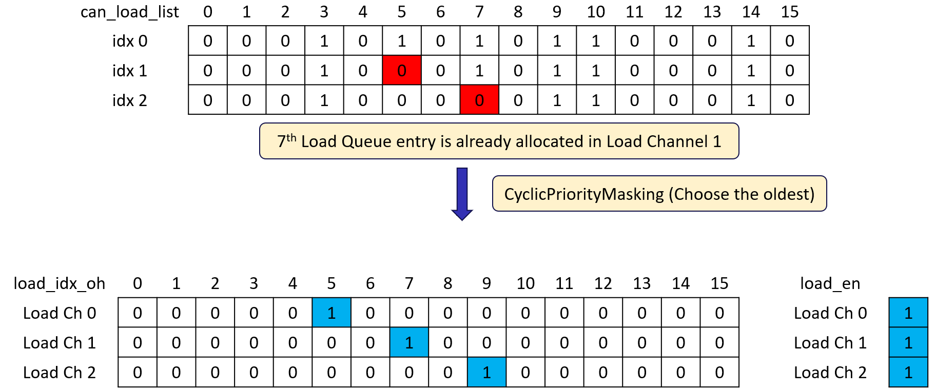
- First, it OR-reduces each row of the
-
Output:
load_en: A vector of enable signals, one for each memory read channel. This directly drivesrreq_valid_o.load_idx_oh: A one-hot vector for each memory channel, identifying which load queue entry won the arbitration. This is used to formrreq_id_oand select therreq_addr_o.
- Store-Load Conflict Logic
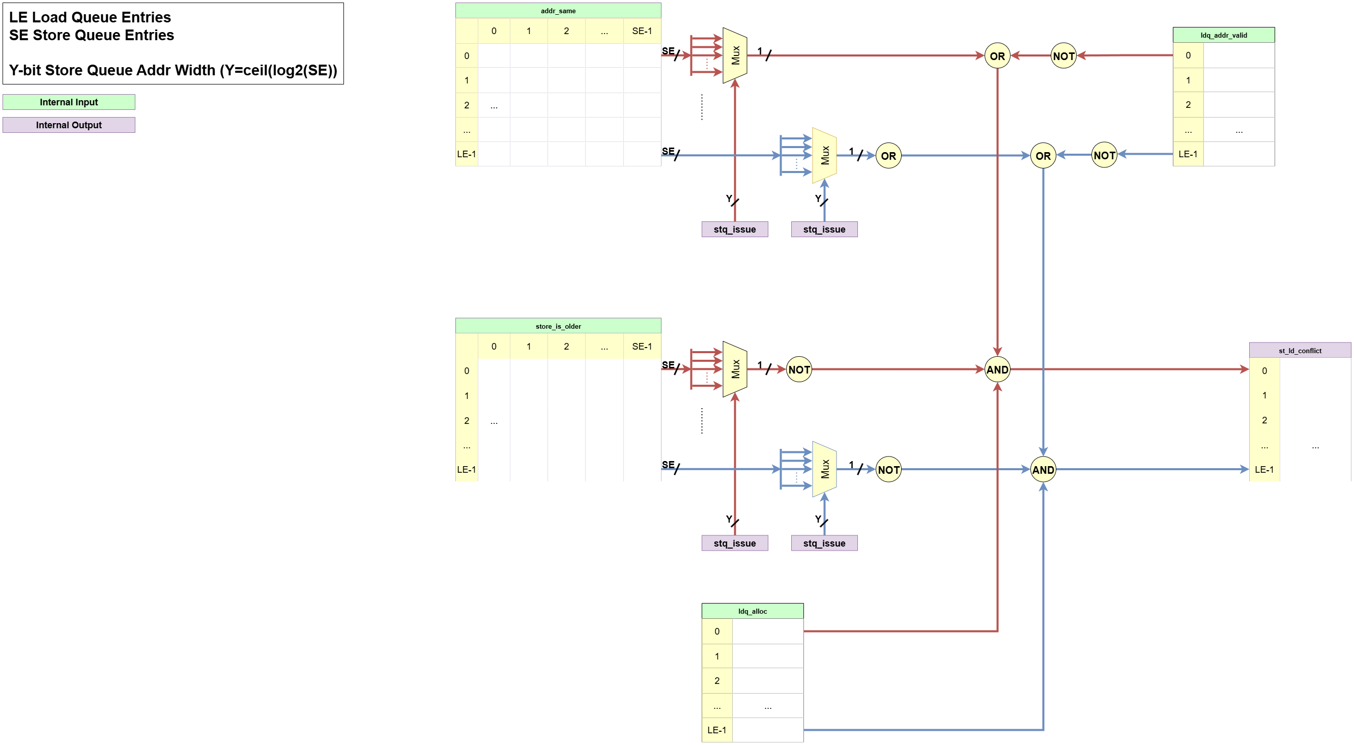 This logic ensures a store operation is not issued if it might conflict with an older, unresolved load operation.
-
Input:
ldq_alloc: A vector indicating which load entries are active.load_completed: A vector indicating whether a load has already received its data from memory.store_is_older: The program order matrix.addr_same: The address equality matrix.ldq_addr_valid: A vector indicating which loads have valid addresses.stq_issue: The pointer to the specific store entry being considered for issue.
-
Processing:
- It checks the store candidate at
stq_issueagainst every active loadi. A conflictst_ld_conflict[i]is asserted if:- The load
iis active (ldq_alloc[i]). - The load
ihas not completed yet (NOT load_completed[i]). - The load
iis older than the store candidate (NOT store_is_older[i][stq_issue]). - A potential address hazard exists, meaning their addresses are identical (
addr_same[i][stq_issue]) OR the load’s address is not yet known (NOT ldq_addr_valid[i]).
- The load
- It checks the store candidate at
-
Output:
st_ld_conflict: A vector indicating which loads are in conflict with the current store candidate. This vector is then OR-reduced to create a singlestore_conflictsignal for the Request Issue Logic.
- Store Queue Bypass Logic (Finalizing the Bypass Decision)
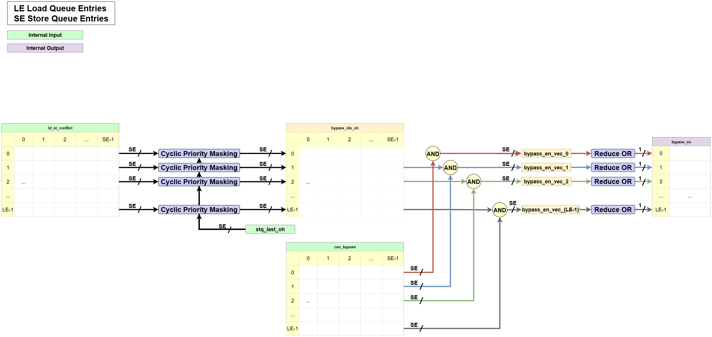 This logic makes the final decision on whether to execute a bypass for a given load.
Note: The bypass logic can be disabled by setting the config parameter
bypasstoFalse. In that case,bypass_enis tied to constant zero, which enables the synthesizer to optimize out the entire bypass logic (including thecan_bypassmatrix). This can significantly lower the LSQ’s resource cost (e.g., by around 50% forhistogramwith 16-entry load and store queues).
-
Input:
ld_st_conflict: The matrix of all load-store dependencies.can_bypass: The matrix of potential bypass opportunities calculated by the Load Queue Bypass Logic.stq_last_oh: A one-hot vector indicating the last allocated store, used for priority.
-
Processing:
- For each load
ithat has conflicts, it usesCyclicPriorityMaskingon its conflict rowld_st_conflict[i]to find the single, youngest store that it depends on. This identifies the store with the most up-to-date data version for that address. - It then checks if a bypass is possible with that specific store by checking the corresponding bit in the
can_bypassmatrix. - If both conditions are met, the bypass is confirmed.
- For each load
-
Output:
bypass_en: A vector wherebypass_en[i]is asserted if loadiwill be satisfied via a bypass in the current cycle. This signal triggers theldq_issue_setand the data muxing from the store queue to the load queue.
- ** Store Issue Stall Logic**
This logic handles a special case that can occur if the store queue is small compared to the memory latency.
In that case, it can happen that all store queue entries have been allocated and are in-flight to memory.
This would case the store issue pointer (
stq_issue) to point to a valid entry (allocated, address valid, and data valid), and would lead to it being issued a second time. To avoid this, we detect the case where the issue pointer (stq_issue) catches up to the tail pointer (stq_tail). If this occurs, store issue is stalled until the tail pointer updates.
-
Input:
stq_issue_next: The store queue issue pointer, plus one.stq_tail: The store queue tail pointer.stq_issue_en: Whether the issue pointer will advance in the next cycle. It is asserted when a store is successfully issued and accepted by the memory interface.stq_tail_update: Whether the tail pointer will update in the next cycle. This is the case when a new group will be allocated that contains at least one store.
-
Processing:
- A single state bit is used to indicate whether store issue is currently stalled.
- The stall bit is set if the next issue pointer equals the tail pointer (
stq_issue_next == stq_tail) and issue is enabled (stq_issue_en). - The stall bit is cleared if the tail pointer updates (
stq_tail_update).
-
Output:
store_issue_stall: Indicates whether store issue is currently stalled.
-
Memory Request Issue Logic This logic is the final stage of the dependency-checking pipeline. It is responsible for arbitrating among safe, ready-to-go memory operations and driving the signals to the external memory interface. It is composed of two distinct parts for handling load and store requests.
14.1. Load Request Issue Logic This part of the logic selects which non-conflicting load requests should be sent to the memory system’s read channels.
-
Input:
ld_st_conflict: The 2D matrix indicating all dependencies between loads and stores.load_req_valid: A vector indicating which loads are active, have a valid address, and have not yet been satisfied.ldq_head_oh: The one-hot head pointer of the load queue, used to grant priority to the oldest requests.ldq_addr: The array of addresses stored in the Load Queue.
-
Processing:
- First, it creates a list of candidate loads (
can_load) by filtering theload_req_validlist, removing any loads that have a dependency indicated by theld_st_conflictmatrix. - It then uses
CyclicPriorityMaskingto arbitrate among thesecan_loadcandidates. This process selects the oldest, highest-priority requests to issue to the available memory read channels.
- First, it creates a list of candidate loads (
-
Output:
rreq_valid_o: The “valid” signal for the memory read request channel. It is asserted when a winning load candidate is selected by the arbitration logic.rreq_addr_o: The address of the winning load, selected from theldq_addrarray via a multiplexer controlled by the arbitration result (load_idx_oh).rreq_id_o: The ID for the read request, which corresponds to the load’s index in the queue. This is also derived from the arbitration result and is used to match the memory response later.
14.2. Store Request Issue Logic This part of the logic determines if the single, oldest pending store request (indicated by the
stq_issuepointer) is safe to send to the memory write channel.-
Input:
st_ld_conflict: A vector indicating if the current store candidate conflicts with any older loads.stq_alloc,stq_addr_valid,stq_data_valid: The status bits for the store entry at thestq_issuepointer.stq_addr,stq_data: The payload data for the store entry at thestq_issuepointer.store_issue_stall: Indicates whether store issue is currently stalled (to avoid wrap-around).
-
Processing:
- It performs a final check to generate the
store_ensignal. The signal is asserted only if the store candidate has no conflicts with older loads (NOT store_conflict) AND its entry is fully prepared (i.e., it is allocated and both its address and data are valid) AND store issue is not stalled (NOT store_issue_stall). - If
store_enis asserted, the logic gates the address and data from the store entry atstq_issueto the write request output ports.
- It performs a final check to generate the
-
Output:
wreq_valid_o: The “valid” signal for the memory write request channel, driven directly by thestore_ensignal.wreq_addr_o,wreq_data_o: The address and data of the store being issued.stq_issue_en: An internal signal that enables thestq_issuepointer to advance. It is asserted when a store is successfully issued and accepted by the memory interface (store_en AND wreq_ready_i).
-
3. Pipelining
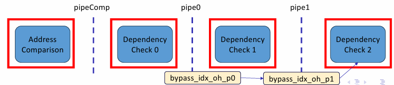
- Purpose
- The dependency-checking unit is the longest combinational path in the LSQ, so we split it into shorter timing-friendly segments.
- Implementation
- Stage 0
pipeComp - Stage 1
pipe0 - Stage 2
pipe1
- Stage 0
Note: Each of these stages can be independently enabled or disabled via the
pipeComp,pipe0, andpipe1config flags—so you only pay the pipeline overhead where you need the extra timing slack.
Group Allocator
This document explains how groups are allocated to the Load-Store Queue (LSQ) in a dataflow circuit.
1. Overview and Purpose
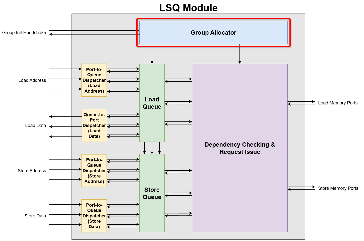
Dataflow circuits have no inherent notion of sequential instructions, and therefore no Fetch or Decode stages. This is a critical problem, because a traditional LSQ relies on this intrinsic program order to resolve potential memory dependencies. Without it, the LSQ is blind.
The solution to this problem is a concept called group allocation. A group is defined as a sequence of memory accesses that are known to execute together, without interruption from control flow. By allocating this entire group into the LSQ at once, we provide the LSQ with the necessary ordering information that was missing.
The Group Allocator is a module that manages entry allocation for the Load-Store Queue (LSQ).
2. Group Allocator Internal Blocks
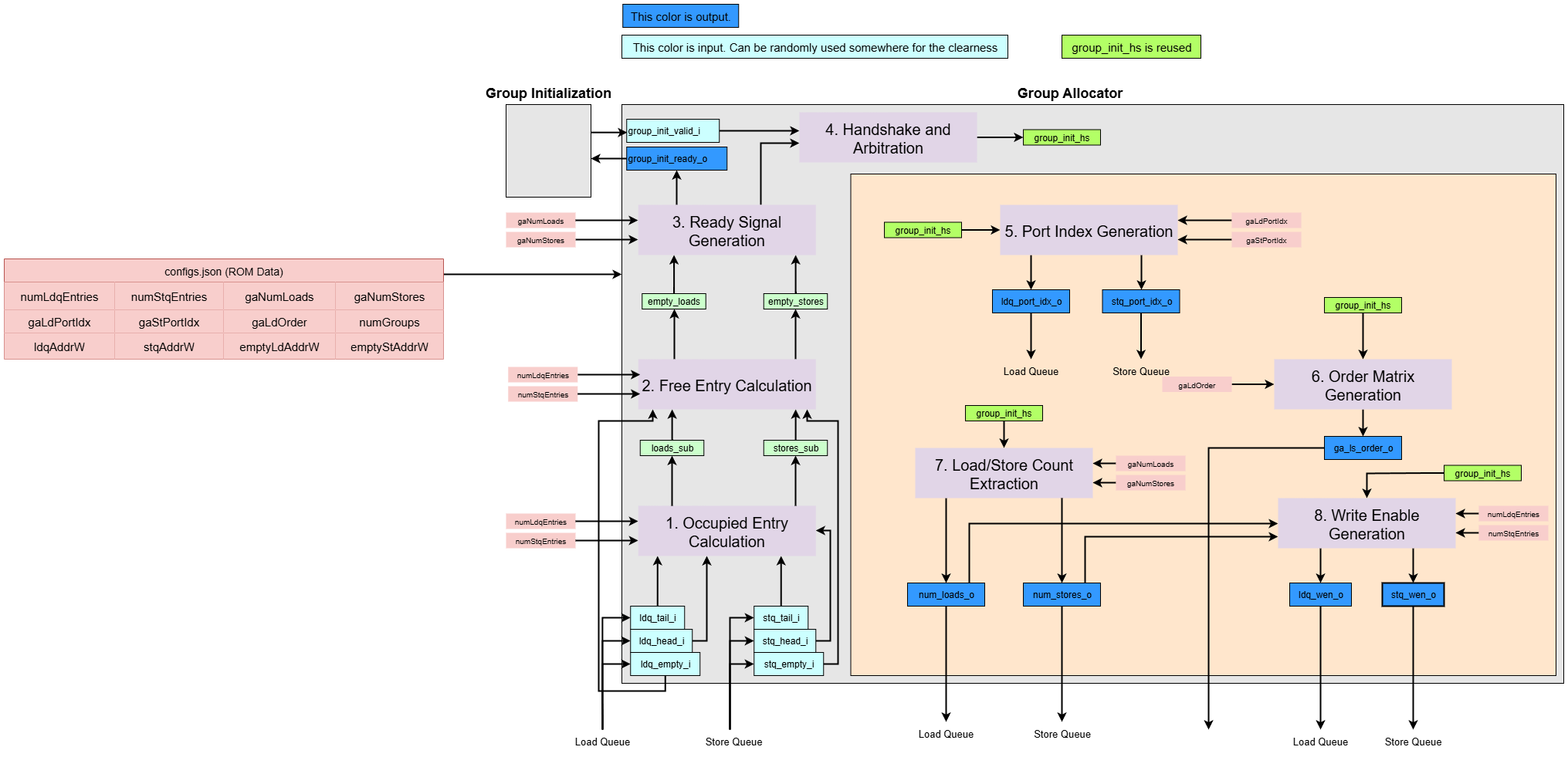
Let’s assume the following generic parameters for dimensionality:
N_GROUPS: The total number of groups.N_LDQ_ENTRIES: The total number of entries in the Load Queue.N_STQ_ENTRIES: The total number of entries in the Store Queue.LDQ_ADDR_WIDTH: The bit-width required to index an entry in the Load Queue (i.e.,ceil(log2(N_LDQ_ENTRIES))).STQ_ADDR_WIDTH: The bit-width required to index an entry in the Store Queue (i.e.,ceil(log2(N_STQ_ENTRIES))).LDP_ADDR_WIDTH: The bit-width required to index the port for a load.STP_ADDR_WIDTH: The bit-width required to index the port for a store.
Signal Naming and Dimensionality:
This module is generated from a higher-level description (e.g., in Python), which results in a specific convention for signal naming in the final VHDL code. It’s important to understand this convention when interpreting diagrams and signal tables.
-
Generation Pattern: A signal that is conceptually an array in the source code (e.g.,
group_init_valid_i) is “unrolled” into multiple, distinct signals in the VHDL entity. The generated VHDL signals are indexed with a suffix, such asgroup_init_valid_{g}_i, where{g}is the group index. -
Interpreting Diagrams: If a diagram or conceptual description uses a base name without an index (e.g.,
group_init_valid_i), it represents a collection of signals. The actual dimension is expanded based on the context:- Group-related signals (like
group_init_valid_i) are expanded by the number of groups (N_GROUPS). - Load queue-related signals (like
ldq_wen_o) are expanded by the number of load queue entries (N_LDQ_ENTRIES). - Store queue-related signals (like
stq_wen_o) are expanded by the number of store queue entries (N_STQ_ENTRIES).
- Group-related signals (like
Interface Signals
In the VHDL Signal Name column, the following placeholders are used: {g} for the group index, {le} for the Load Queue entry index, and {se} for the Store Queue entry index.
| Python Variable Name | VHDL Signal Name | Direction | Dimensionality | Description |
|---|---|---|---|---|
| Inputs | ||||
group_init_valid_i | group_init_valid_{g}_i | Input | std_logic | Valid signal indicating a request to allocate group g. |
ldq_tail_i | ldq_tail_i | Input | std_logic_vector(LDQ_ADDR_WIDTH-1:0) | Current tail pointer of the Load Queue. |
ldq_head_i | ldq_head_i | Input | std_logic_vector(LDQ_ADDR_WIDTH-1:0) | Current head pointer of the Load Queue. |
ldq_empty_i | ldq_empty_i | Input | std_logic | A flag indicating if the Load Queue is empty. |
stq_tail_i | stq_tail_i | Input | std_logic_vector(STQ_ADDR_WIDTH-1:0) | Current tail pointer of the Store Queue. |
stq_head_i | stq_head_i | Input | std_logic_vector(STQ_ADDR_WIDTH-1:0) | Current head pointer of the Store Queue. |
stq_empty_i | stq_empty_i | Input | std_logic | A flag indicating if the Store Queue is empty. |
| Outputs | ||||
group_init_ready_o | group_init_ready_{g}_o | Output | std_logic | Ready signal indicating the allocator can accept a request for group g. |
ldq_wen_o | ldq_wen_{le}_o | Output | std_logic | Write enable signal for Load Queue entry {le}. |
num_loads_o | num_loads_o | Output | std_logic_vector(LDQ_ADDR_WIDTH-1:0) | The number of loads in the newly allocated group. |
ldq_port_idx_o | ldq_port_idx_{le}_o | Output | std_logic_vector(LDP_ADDR_WIDTH-1:0) | The source port index for the operation to be written into Load Queue entry {le}. |
stq_wen_o | stq_wen_{se}_o | Output | std_logic | Write enable signal for Store Queue entry {se}. |
num_stores_o | num_stores_o | Output | std_logic_vector(STQ_ADDR_WIDTH-1:0) | The number of stores in the newly allocated group. |
stq_port_idx_o | stq_port_idx_{se}_o | Output | std_logic_vector(STP_ADDR_WIDTH-1:0) | The source port index for the operation to be written into Store Queue entry {se}. |
ga_ls_order_o | ga_ls_order_{le}_o | Output | std_logic_vector(N_STQ_ENTRIES-1:0) | For the load in a load queue entry {le}, this vector indicates its order dependency relative to all store queue entries. |
The Group Allocator has the following responsibilities:
-
Preliminary Free Entry Calculator
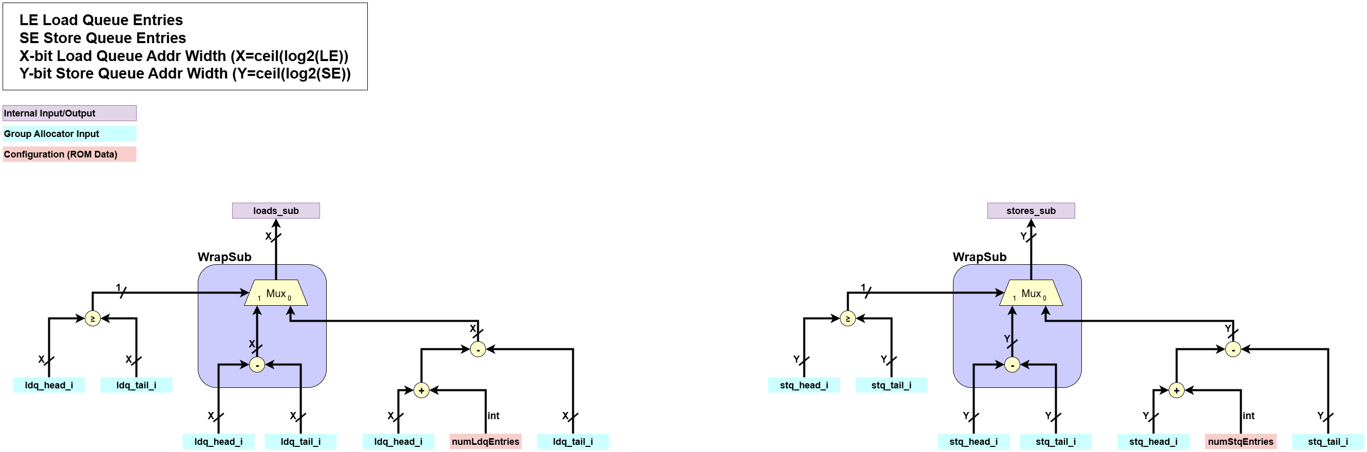
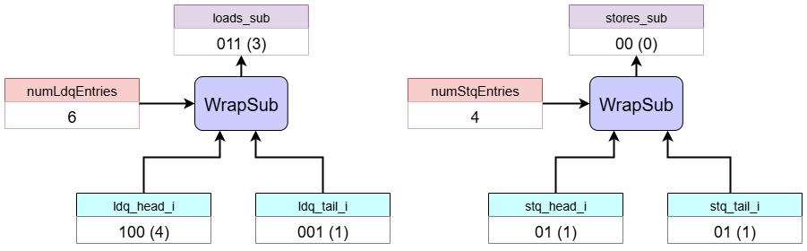
This block performs an initial calculation of the number of free entries in each queue.- Input:
ldq_head_i,ldq_tail_i: Head and tail pointers for the Load Queue.stq_head_i,stq_tail_i: Head and tail pointers for the Store Queue.
- Processing:
- It performs a cyclic subtraction (
WrapSub) of the pointers for each queue. This calculation gives the number of empty slots but is ambiguous when the two pointers are the same (head == tail) since it can either mean empty or full.if head >= tail: out = head - tail else: out = (head + numEntries) - tail
- It performs a cyclic subtraction (
- Output:
loads_sub,stores_sub: Intermediate signals holding the result of the cyclic subtraction for each queue.
- Input:
-
Free Entry Calculation
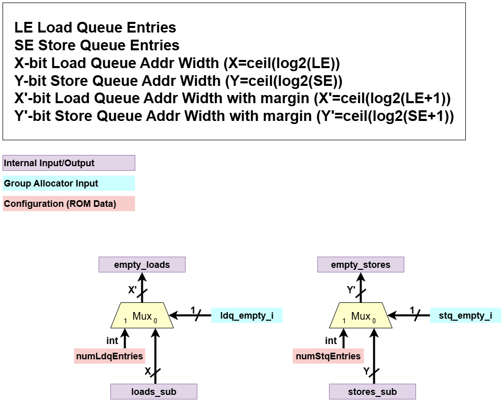
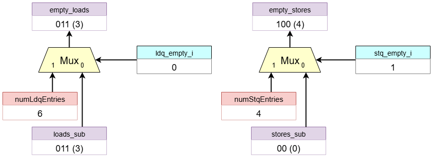
This block determines the final number of free entries available in each queue.- Input:
loads_sub,stores_sub: The tentative free entry counts from the previous block.ldq_empty_i,stq_empty_i: Flags indicating if each queue is empty.
- Processing:
- It uses multiplexer logic to resolve the ambiguity of the previous step.
- If a queue’s
emptyflag is asserted, it outputs the maximum queue size (numLdqEntriesornumStqEntries). - Otherwise, it outputs the result from the
WrapSubcalculation.
- Output:
empty_loads,empty_stores: The definitive number of free entries in the load and store queues.
- Input:
-
Ready Signal Generation
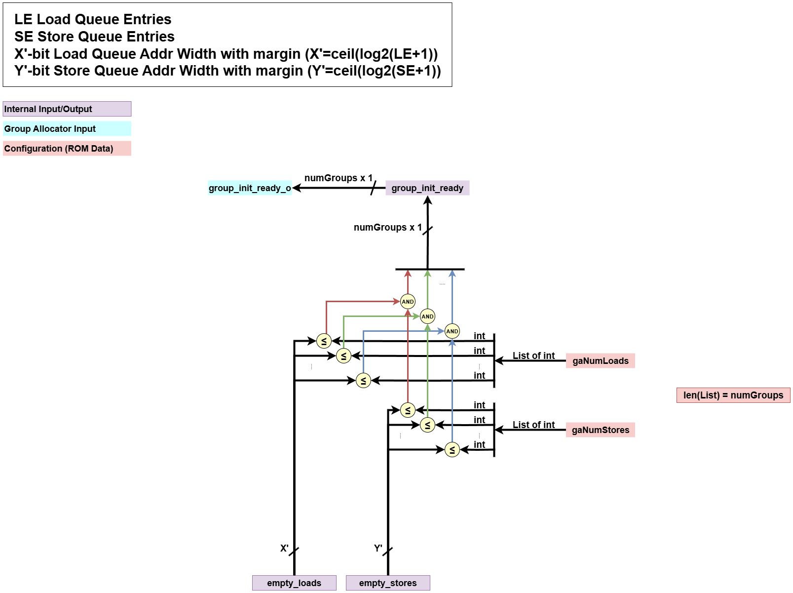
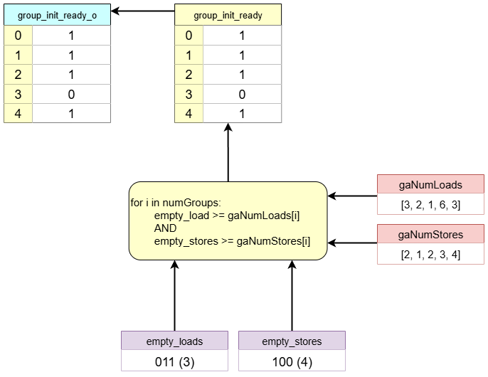
This block checks if there is sufficient space in the queues for each potential group.- Input:
empty_loads,empty_stores: The number of free entries available in each queue.gaNumLoads,gaNumStores: Configuration arrays specifying the number of loads and stores required by each group.
- Processing:
- For each group, it compares the available space (
empty_loads,empty_stores) with the required space (gaNumLoads[g],gaNumStores[g]). - A group is considered “ready” only if there is enough space for both its loads and its stores.
- For each group, it compares the available space (
- Output:
group_init_ready: An array of ready signals, one for each group, indicating whether it could be allocated.group_init_ready_o: The final ready signals sent to the external logic.
- Input:
-
Handshake and Arbitration
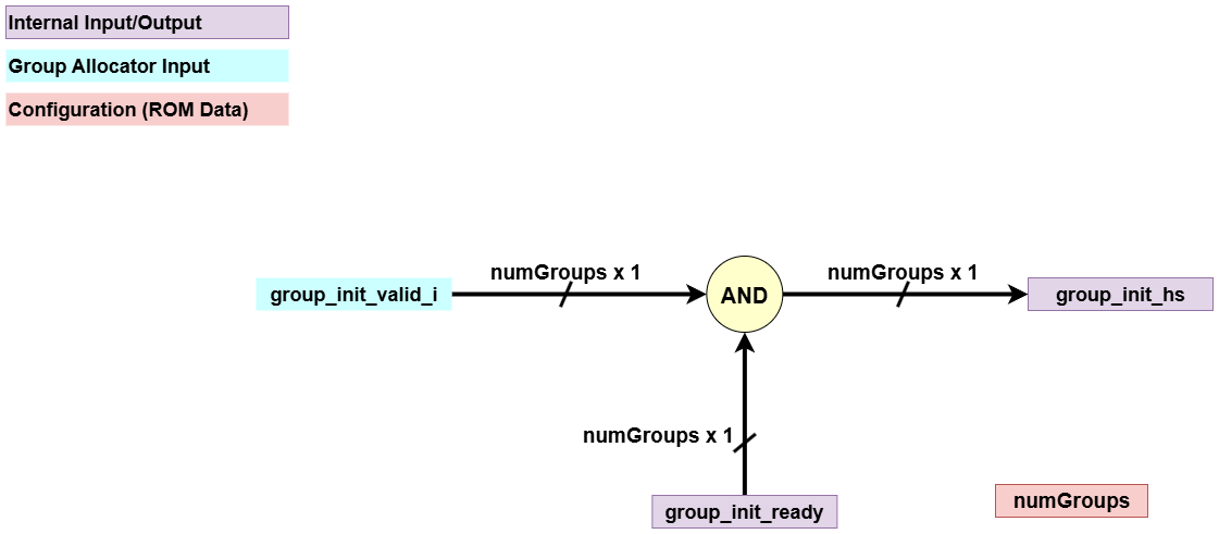
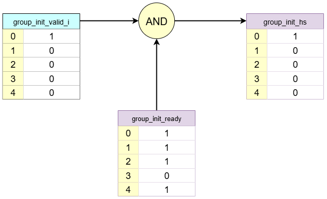
This block performs the final handshake to select a single allocated group for the current cycle. However, the arbitration happens when one of the configuration signalgaMultiis on, and this diagram depicts whengaMultiis off.- Input:
group_init_ready: The readiness status for each group from the previous block.group_init_valid_i: The external valid signals for each group.- (Optional)
ga_rr_mask: A round-robin mask used for arbitration if multiple groups can be allocated (gaMultiis true).
- Processing:
- It combines the
readyandvalidsignals. A group must be both ready and valid to be a candidate for allocation. - If multiple groups are candidates, an arbitrator (e.g.,
CyclicPriorityMasking) selects a single group. IfgaMultiis false, it assumes only one valid allocation request can occur at a time as depicted.
- It combines the
- Output:
group_init_hs: A one-hot signal indicating the single group that will be allocated at the current cycle.
- Input:
-
Port Index Generation
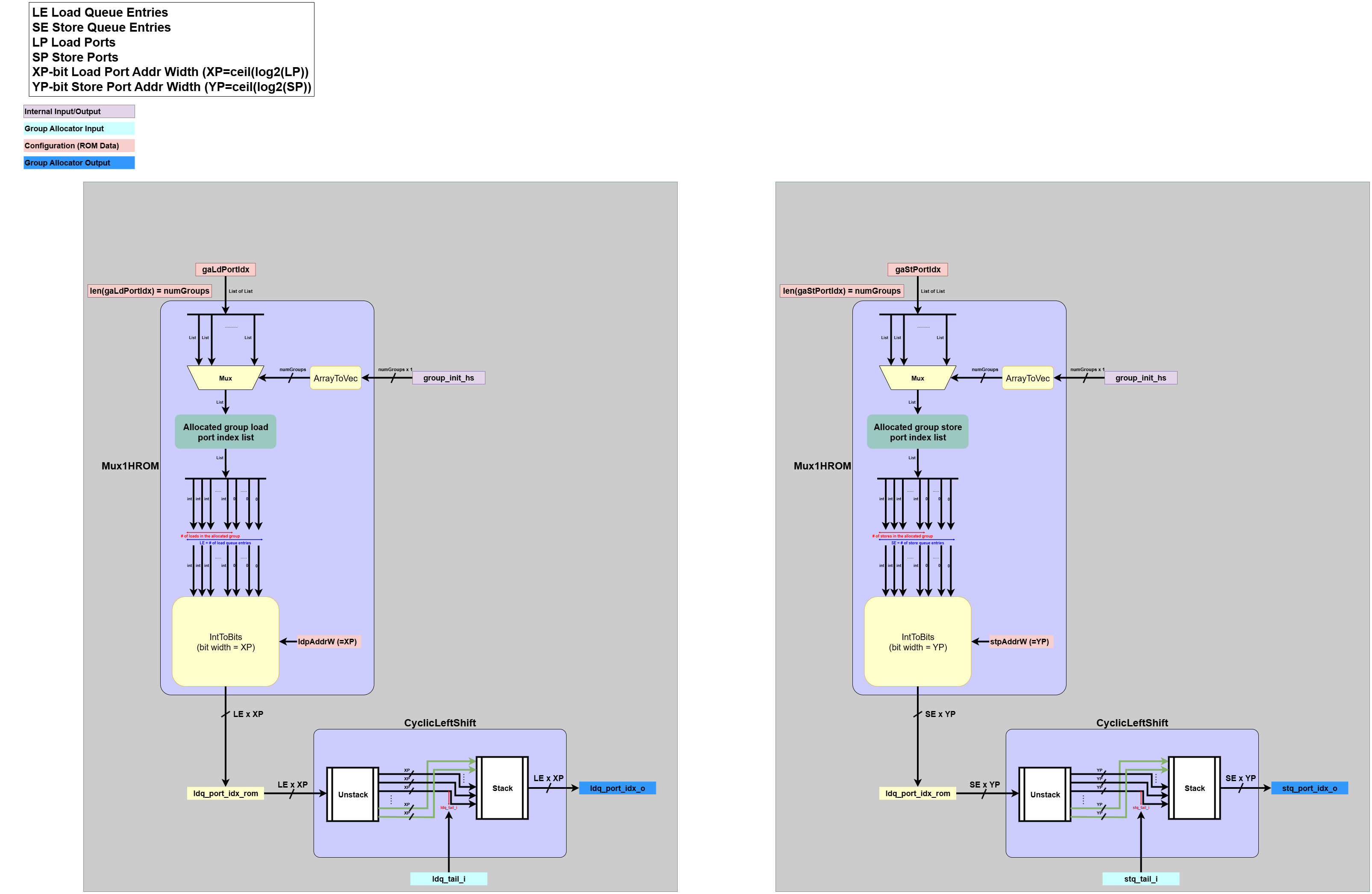
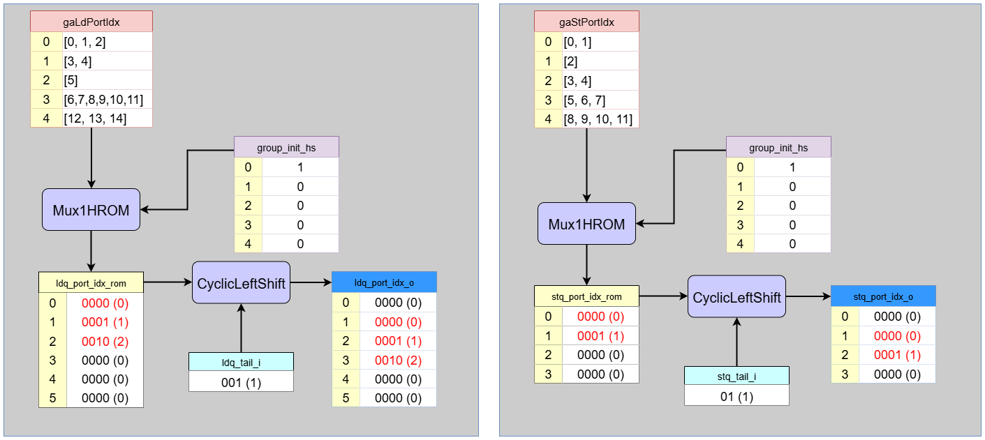
This block generates the correctly aligned port indices for the entries being allocated.- Input:
group_init_hs: A one-hot signal indicating the single group that will be allocated at the current cycle.ldq_tail_i,stq_tail_i: The current tail pointers of the queues.gaLdPortIdx,gaStPortIdx: Pre-compiled ROMs containing the port indices for each group.
- Processing:
- Uses the
group_init_hssignal to perform a ROM lookup (Mux1HROM), selecting the list of port indices for the allocated group. - Performs
CyclicLeftShifton the selected list, using the corresponding queue’stailpointer as the shift amount. This aligns the indices to the correct physical queue entry slots.
- Uses the
- Output:
ldq_port_idx_o,stq_port_idx_o: The final, shifted port indices to be written into the newly allocated queue entries.
- Input:
-
Order Matrix Generation
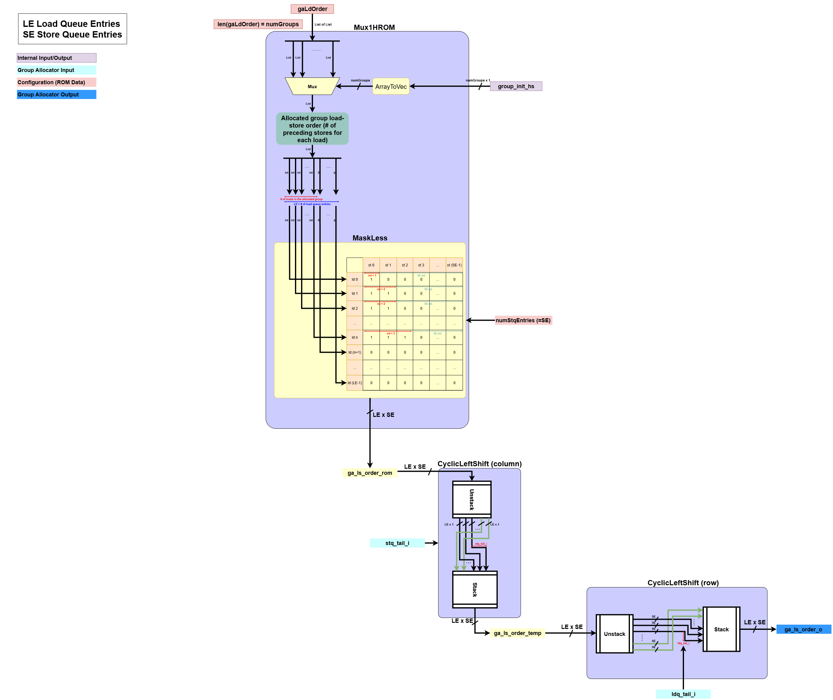
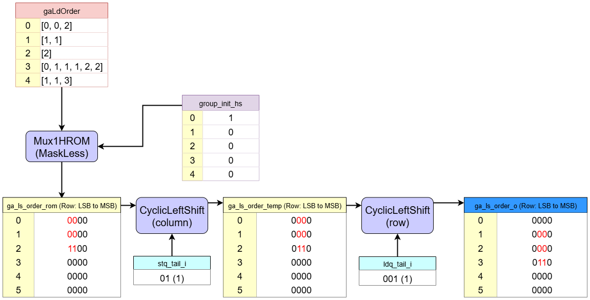
This block generates the load-store order matrix between the new loads and stores in the allocated group.- Input:
group_init_hs: A one-hot signal indicating the single group that will be allocated at the current cycle.ldq_tail_i,stq_tail_i: The current tail pointers of the queues.gaLdOrder: A pre-compiled ROM containing the load-store order information for each group. For each group, the corresponding list indicates, from the perspective of a load, the number of stores that come before it within the same group.
- Processing:
- Uses
group_init_hsto perform a ROM lookup, selecting the order information for the allocated group. This information is used to build an un-aligned load-store order matrix. - A
1in(le, se)indicates thatstore_{se}comes beforeload_{le}. This is built by the functionMaskLess. - Performs
CyclicLeftShifton this matrix two times, shifting it horizontally bystq_tail_iand vertically byldq_tail_i. This correctly places the sub-matrix within the LSQ’s main order matrix.
- Uses
- Output:
ga_ls_order_o: The final, shifted load-store order matrix defining the order of the new loads and stores.
- Input:
-
Load/Store Count Extraction
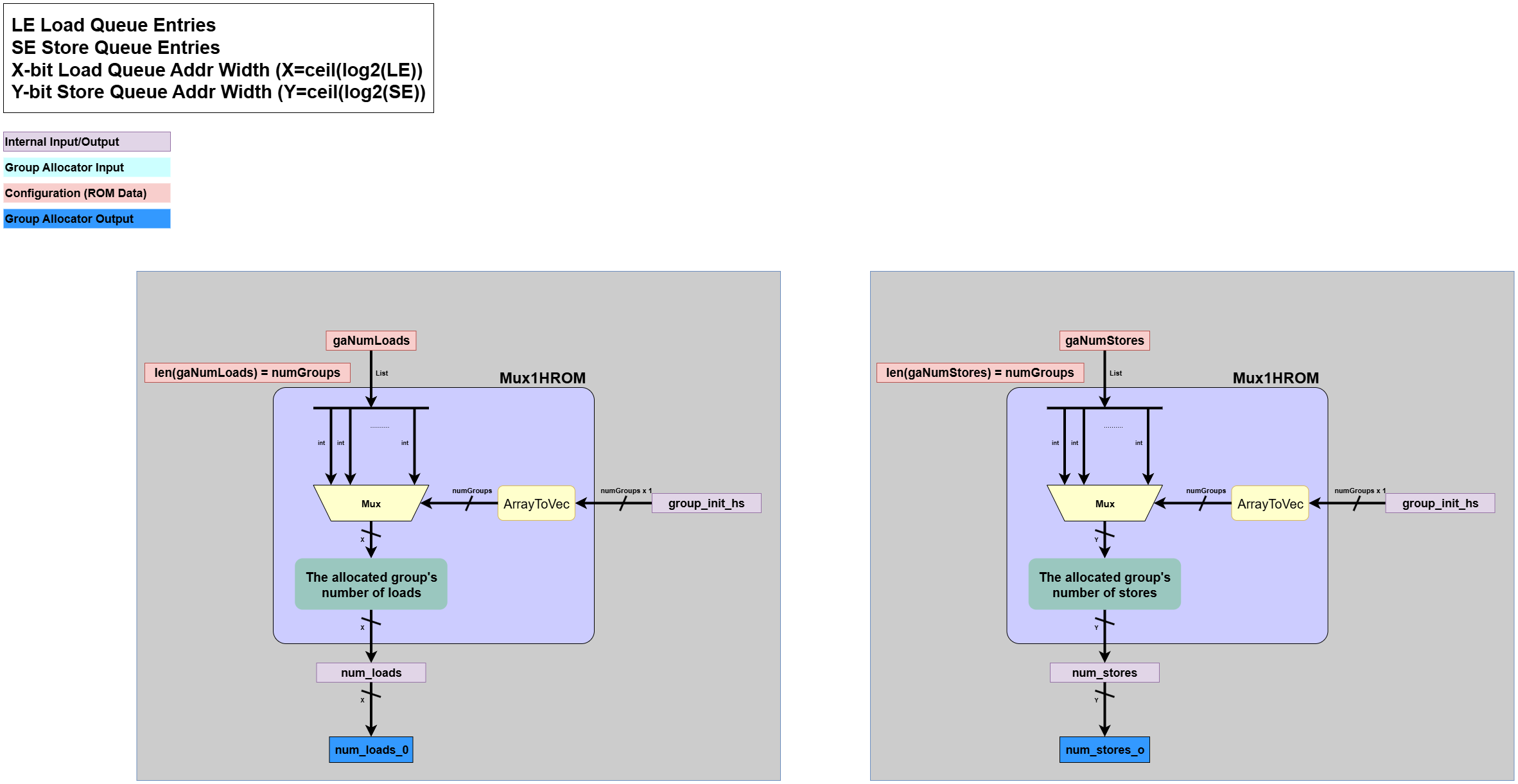
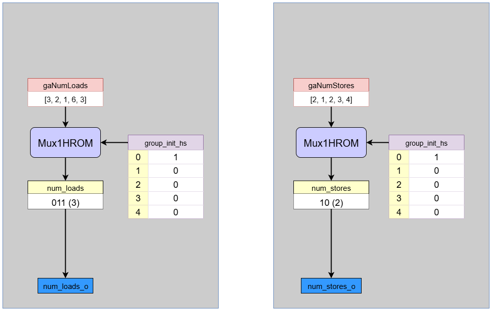
This block extracts the number of loads and stores for the allocated group.- Input:
group_init_hs: A one-hot signal indicating the single group that will be allocated at the current cycle.gaNumLoads,gaNumStores: Pre-compiled ROMs containing the load/store counts for each group.
- Processing:
- Performs a simple ROM lookup (
Mux1HROM) usinggroup_init_hsto select the number of loads and stores corresponding to the allocated group.
- Performs a simple ROM lookup (
- Output:
num_loads_o,num_stores_o: The number of loads and stores in the newly allocated group.
- Input:
-
Write Enable Generation
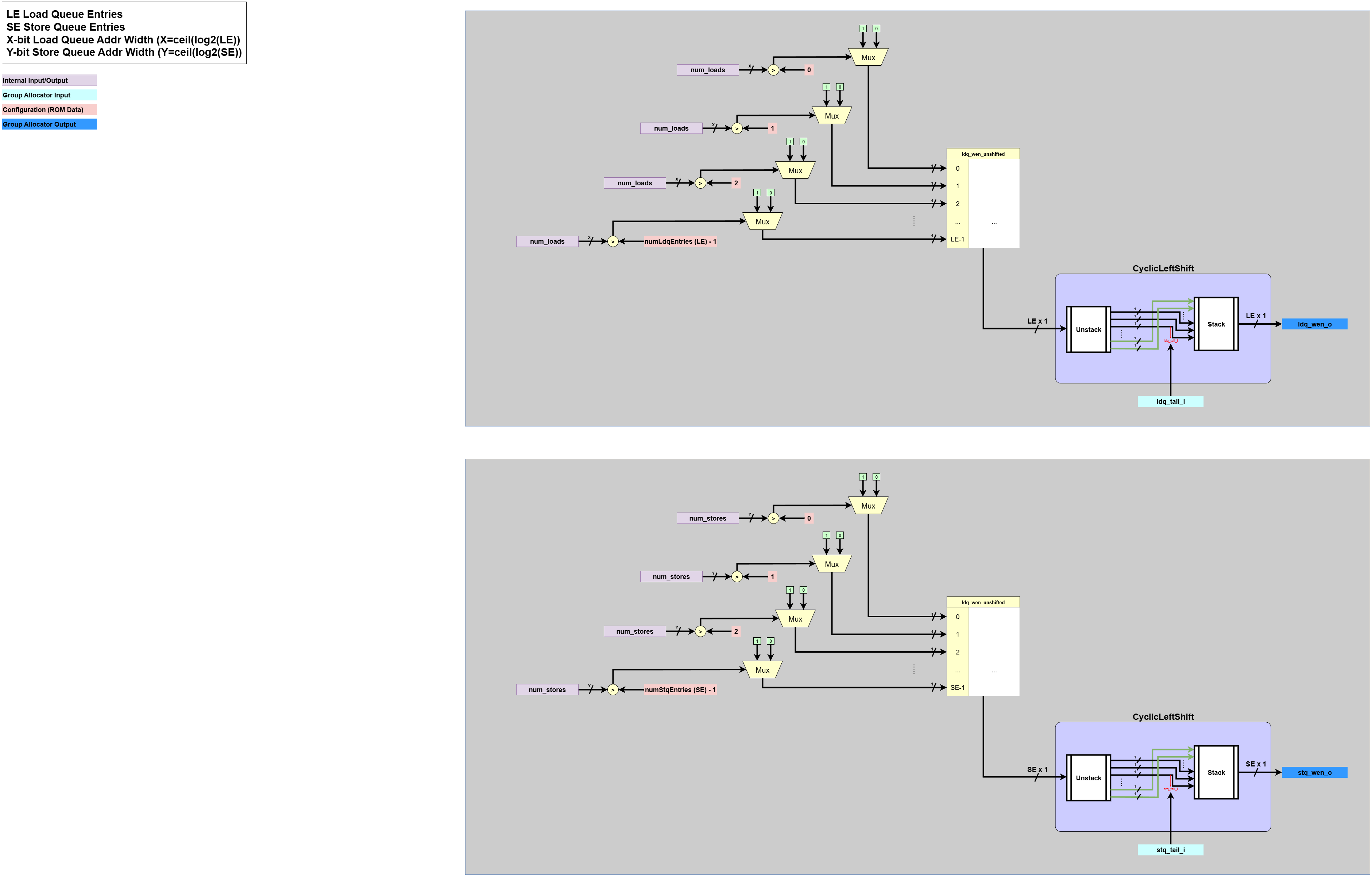
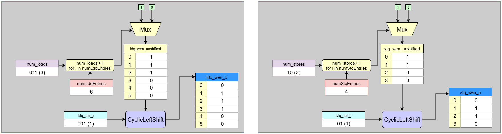
This final block generates the write-enable signals to allocate the new queue entries.- Input:
num_loads,num_stores: The load/store counts from the previous block.ldq_tail_i,stq_tail_i: The current tail pointers of the queues.
- Processing:
- First, it creates an unshifted bitmask. For example, if
num_loadsis 3, the mask is...00111. - It then applies
CyclicLeftShiftto this mask, using the queue’stailpointer as the shift amount. This rotates the block of1s to start at thetailposition.
- First, it creates an unshifted bitmask. For example, if
- Output:
ldq_wen_o,stq_wen_o: The final write-enable vectors, which assert a ‘1’ for the precise entries in each queue that are being allocated.
- Input:
3. Dataflow Walkthrough
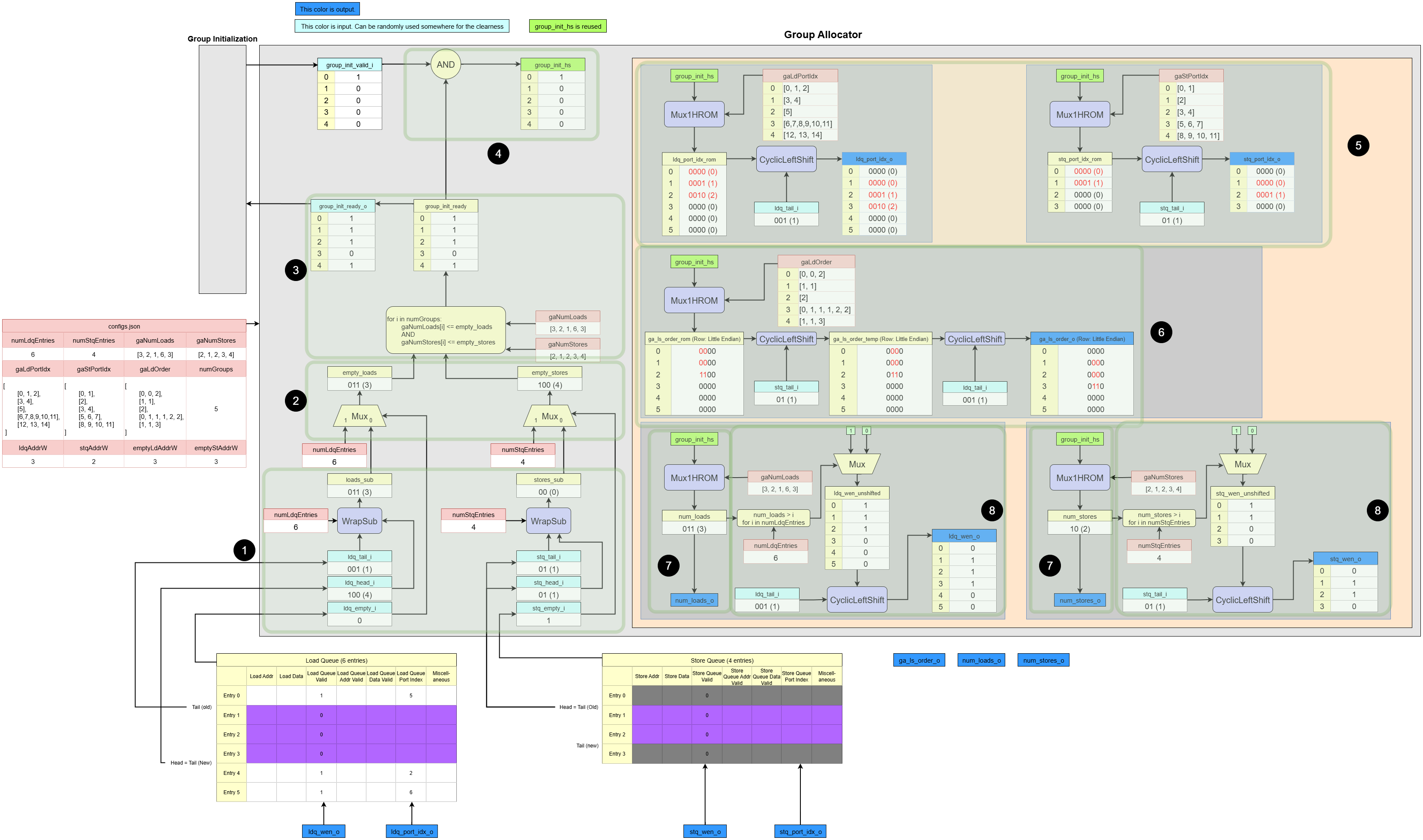
Example of Group Allocator
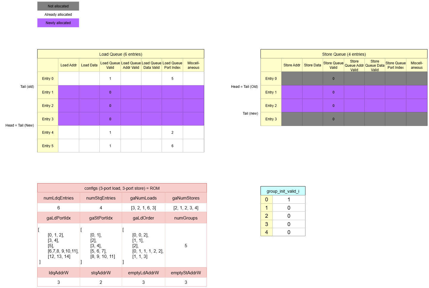
This walkthrough explains the step-by-step operation of the Group Allocator based on the following precise initial state:
- Queue State:
- Load Queue:
ldq_tail=1,ldq_head=4,ldq_empty_i=0 (Not Empty) - Store Queue:
stq_tail=1,stq_head=1,stq_empty_i=1 (Empty)
- Load Queue:
- Queue Sizes:
numLdqEntries=6,numStqEntries=4 - Group Allocation Request:
group_init_valid_i=[1,0,0,0,0](Only Group 0 is requesting the allocation) - Group Configurations:
gaNumLoads=[3, 2, 1, 6, 3]gaNumStores=[2, 1, 2, 3, 4]
1. Preliminary Free Entry Calculation
This block calculates the tentative number of currently free entries in each queue.
- Load Queue: It performs a cyclic subtraction
ldq_head(4) -ldq_tail(1) =3. There are 3 free entries. - Store Queue: It performs a cyclic subtraction
stq_head(1) -stq_tail(1) =0. However, there are actually4free entries instead of0. This result is ambiguous and will be resolved in the next step.
2. Free Entry Calculation
This block calculates the number of available empty entries.
- Load Queue: Since
ldq_empty_iis0(false), there are 3 free entries in the load queue. - Store Queue: Since
stq_empty_iis1(true), it outputs the total queue size. There are 4 free entries in the Store Queue.
3. Ready Signal Generation
This block checks if the load queue and store queue are ready to be allocated.
- Required Space for Group 0:
gaNumLoads[0]=3,gaNumStores[0]=2.- Comparison:
- Loads: Is free space (3) >= required space (3)? Yes.
- Stores: Is free space (4) >= required space (2)? Yes.
group_init_ready[0] = 1
- Comparison:
- Required Space for Group 1:
gaNumLoads[1]=2,gaNumStores[1]=1.- Comparison:
- Loads: Is free space (3) >= required space (2)? Yes.
- Stores: Is free space (4) >= required space (1)? Yes.
group_init_ready[1] = 1
- Comparison:
- Required Space for Group 2:
gaNumLoads[2]=1,gaNumStores[2]=2.- Comparison:
- Loads: Is free space (3) >= required space (1)? Yes.
- Stores: Is free space (4) >= required space (2)? Yes.
group_init_ready[2] = 1
- Comparison:
- Required Space for Group 3:
gaNumLoads[3]=6,gaNumStores[3]=3.- Comparison:
- Loads: Is free space (3) >= required space (6)? No.
- Stores: Is free space (4) >= required space (3)? Yes.
group_init_ready[3] = 0
- Comparison:
- Required Space for Group 4:
gaNumLoads[4]=3,gaNumStores[4]=4.- Comparison:
- Loads: Is free space (3) >= required space (3)? Yes.
- Stores: Is free space (4) >= required space (4)? Yes.
group_init_ready[4] = 1
- Comparison:
4. Handshake and Arbitration
This block performs the handshake to select an allocated group.
- The incoming request
group_init_valid_iis[1,0,0,0,0]. - The
readysignal for Group 0 is1. - The AND result is
[1,0,0,0,0], and since only one request is active, Group 0 is allocated.
5. Port Index Generation
This block generates the correctly aligned port indices for the newly allocated entries. It first looks up the data for the allocated group (Group 0), pads it to the full queue length, and then performs the specified shift operation to align it with the tail pointer.
-
Load Port Index (
ldq_port_idx_o):- ROM Lookup: It fetches
gaLdPortIdx[0], which is[0, 1, 2]. This means thatload0_0(Group0’s 0th load),load0_1(Group0’s 1st load), andload0_2(Group0’s 2nd load) usePort 0,Port 1, andPort 2respectively. Since the load queue has 6 entries, this is padded to create the intermediate vectorldq_port_idx_rom = [0, 1, 2, 0, 0, 0]. - Alignment: These indices must be placed into the physical queue entries starting at
ldq_tail=1.- Physical
Entry 1gets Port Index0. - Physical
Entry 2gets Port Index1. - Physical
Entry 3gets Port Index2.
- Physical
- Final Vector: The resulting vector of port indices is
[0, 0, 1, 2, 0, 0]. (Note: This vector represents the indices[?, 0, 1, 2, ?, ?]aligned to the 6 queue entries, with unused entries being 0).
- ROM Lookup: It fetches
-
Store Port Index (
stq_port_idx_o):- ROM Lookup: It fetches
gaStPortIdx[0], which is[0, 1]. This is padded to the 4-entry store queue length to become[0, 1, 0, 0]. - Alignment: These are placed starting at
stq_tail=1.- Physical
Entry 1gets Port Index0. - Physical
Entry 2gets Port Index1.
- Physical
- Final Vector: The resulting vector is
[0, 0, 1, 0]. (Note: This represents[?, 0, 1, ?]aligned to the 4 queue entries).
- ROM Lookup: It fetches
6. Order Matrix Generation
This block fetches the intra-group order matrix for Group 0 and aligns it.
-
ROM Lookup: It retrieves
gaLdOrder[0], which is[0, 0, 2]. This defines the intra-group dependencies for the group0:Load 0: There are 0 stores before it.Load 1: There are 0 stores before it.Load 2: There are 2 stores before it (Store 0andStore 1).- This creates a
3x2dependency sub-matrix:s0 s1 l0 [0, 0] l1 [0, 0] l2 [1, 1]
For this, the order matrix becomes
ga_ls_order_rom SQ0 SQ1 SQ2 SQ3 LQ Entry 0: [ 0, 0, 0, 0 ] LQ Entry 1: [ 0, 0, 0, 0 ] LQ Entry 2: [ 1, 1, 0, 0 ] LQ Entry 3: [ 0, 0, 0, 0 ] LQ Entry 4: [ 0, 0, 0, 0 ] LQ Entry 5: [ 0, 0, 0, 0 ] -
Matrix Alignment: This
3x2sub-matrix is placed into the final6x4ga_ls_order_omatrix, with its top-left corner aligned to(ldq_tail, stq_tail)which is(1, 1). The new loads occupy physical entries {1, 2, 3} and new stores occupy {1, 2}. The dependency of Load 2 (physical entry 3) on Store 0 (physical entry 1) and Store 1 (physical entry 2) is mapped accordingly. -
Final Matrix (
ga_ls_order_o): The final matrix will have1s atga_ls_order_o[3][1]andga_ls_order_o[3][2]. All other entries related to this group are0.SQ0 SQ1 SQ2 SQ3 LQ Entry 0: [ 0, 0, 0, 0 ] LQ Entry 1: [ 0, 0, 0, 0 ] // New Load 0 LQ Entry 2: [ 0, 0, 0, 0 ] // New Load 1 LQ Entry 3: [ 0, 1, 1, 0 ] // New Load 2 depends on new Store 0 & 1 LQ Entry 4: [ 0, 0, 0, 0 ] LQ Entry 5: [ 0, 0, 0, 0 ]
7. Load/Store Count Extraction
This block extracts the number of loads and stores for the allocated group (Group 0).
- ROM Lookup: It retrieves
gaNumLoads[0](3) andgaNumStores[0](2). - The outputs
num_loads_oandnum_stores_obecome3and2, respectively.
8. Write Enable Generation
This final block generates the write-enable signals that allocate the newly allocated queue entries.
- Unshifted Mask Creation:
- Loads:
num_loads(3) creates a 6-bit unshifted mask000111. - Stores:
num_stores(2) creates a 4-bit unshifted mask0011.
- Loads:
- Cyclic Left Shift:
ldq_wen_o: The mask000111is shifted byldq_tail(1), resulting in001110.stq_wen_o: The mask0011is shifted bystq_tail(1), resulting in0110.
- These final vectors assert ‘1’ for entries 1, 2, 3 in the Load Queue and entries 1, 2 in the Store Queue, activating them for the new group.
Port-to-Queue Dispatcher
How addresses and data enter from multiple access ports to the LSQ’s internal load and store queues.
1. Overview and Purpose
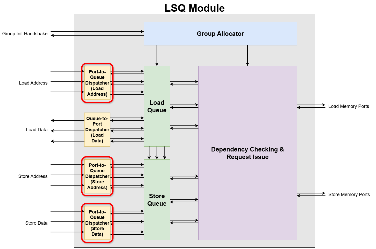
The Port-to-Queue Dispatcher is a submodule within the Load-Store Queue (LSQ) responsible for routing incoming memory requests (addresses or data) from the dataflow circuit’s access ports to the correct queue entries of the load queue and the store queue. All incoming requests are directed into either the load queue or the store queue. These queues are essential for tracking every memory request until its completion. It ensures each load queue or store queue entry gets the correct address or data from the appropriate port.
We need a total of three Port-to-Queue Dispatchers—one each for the load address, store address, and store data. Why? To load, you must first supply the address where the data is stored. Likewise, a store operation needs both the value to write and the address to write it at.
In the LSQ architecture, memory operations arrive via dedicated access ports. The system can process simultaneous payload writes to the LSQ from multiple ports in parallel. An arbitration mechanism is required, however, to handle cases where multiple queue entries compete for access to the same single port.
2. Port-to-Queue Dispatcher Internal Blocks
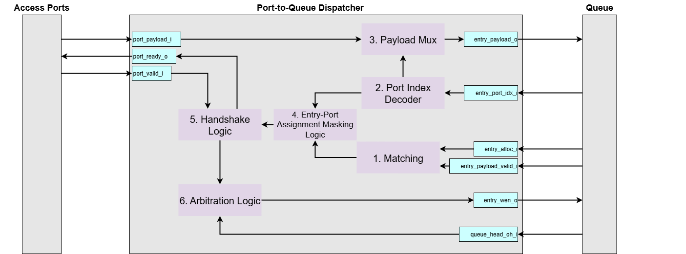
Let’s assume the following generic parameters for dimensionality:
N_PORTS: The total number of ports.N_ENTRIES: The total number of entries in the queue.PAYLOAD_WIDTH: The bit-width of the payload (e.g., 8 bits).PORT_IDX_WIDTH: The bit-width required to index a port (e.g.,ceil(log2(N_PORTS))).
Signal Naming and Dimensionality:
This module is generated from a higher-level description (e.g., in Python), which results in a specific convention for signal naming in the final VHDL code. It’s important to understand this convention when interpreting diagrams and signal tables.
-
Generation Pattern: A signal that is conceptually an array in the source code (e.g.,
port_payload_i) is “unrolled” into multiple, distinct signals in the VHDL entity. The generated VHDL signals are indexed with a suffix, such asport_payload_{p}_i, where{p}is the port index. -
Interpreting Diagrams: If a diagram or conceptual description uses a base name without an index (e.g.,
port_payload_i), it represents a collection of signals. The actual dimension is expanded based on the context:- Port-related signals (like
port_payload_i) are expanded by the number of ports (N_PORTS). - Entry-related signals (like
entry_alloc_i) are expanded by the number of queue entries (N_ENTRIES).
- Port-related signals (like
Port Interface Signals
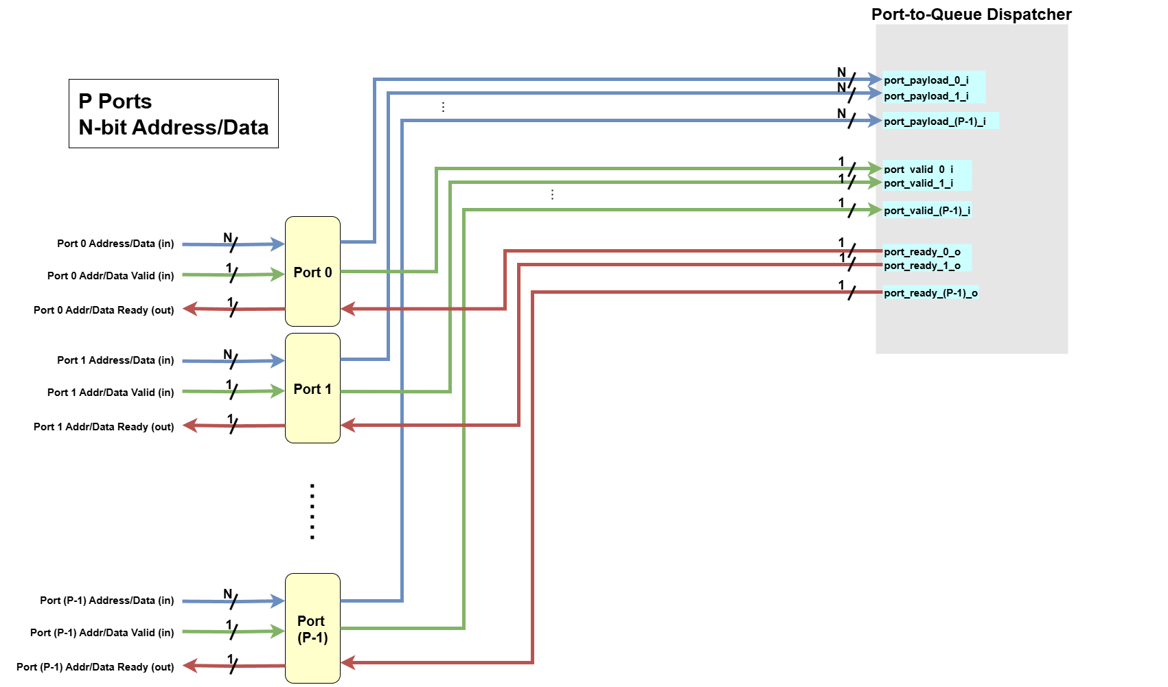
These signals are used for communication between the external modules and the dispatcher’s ports.
p=[0, N_PORTS-1]
| Python Variable Name | VHDL Signal Name | Direction | Dimensionality | Description |
|---|---|---|---|---|
| Inputs | ||||
port_payload_i | port_payload_{p}_i | Input | std_logic_vector(PAYLOAD_WIDTH-1:0) | The payload (address or data) for port p. |
port_valid_i | port_valid_{p}_i | Input | std_logic | Valid flag for port p. When high, it indicates that the payload on port_payload_{p}_i is valid. |
| Outputs | ||||
port_ready_o | port_ready_{p}_o | Output | std_logic | Ready flag for port p. This signal goes high if the queue can accept the payload from port p this cycle. |
Queue Interface Signals
These signals are used for communication between the dispatcher logic and the queue’s memory entries.
e=[0, N_ENTRIES-1]
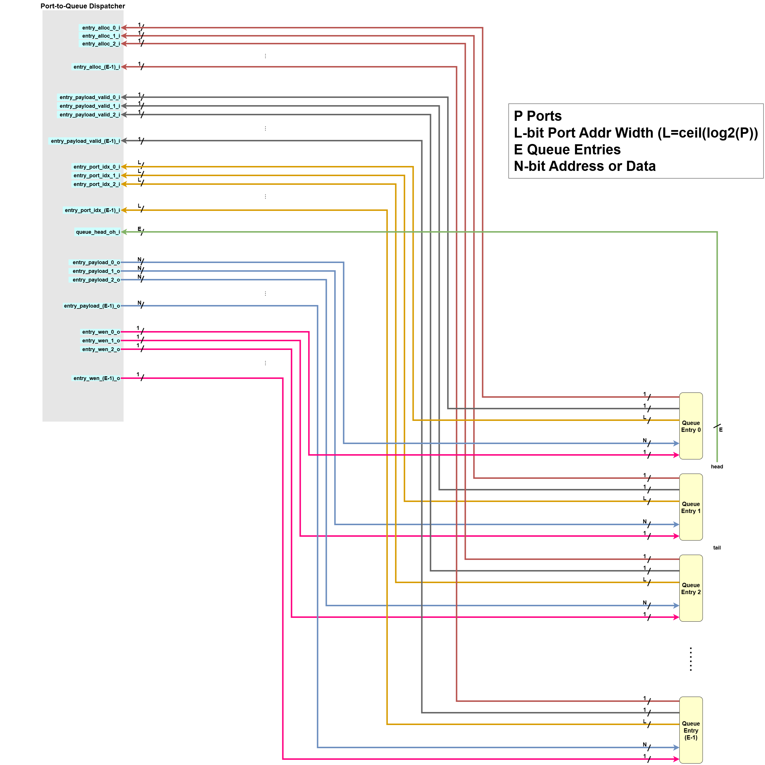
| Python Variable Name | VHDL Signal Name | Direction | Dimensionality | Description |
|---|---|---|---|---|
| Inputs | ||||
entry_alloc_i | entry_alloc_{e}_i | Input | std_logic | Is queue entry e logically allocated? |
entry_payload_valid_i | entry_payload_valid_{e}_i | Input | std_logic | Indicates if the entry’s payload slot e is already valid. |
entry_port_idx_i | entry_port_idx_{e}_i | Input | std_logic_vector(PORT_IDX_WIDTH-1:0) | Indicates to which port entry e is assigned. |
queue_head_oh_i | queue_head_oh_{e}_i | Input | std_logic_vector(N_ENTRIES-1:0) | One-hot vector indicating the head entry in the queue. |
| Outputs | ||||
entry_payload_o | entry_payload_{e}_o | Output | std_logic_vector(PAYLOAD_WIDTH-1:0) | The payload to be written into queue entry e. |
entry_wen_o | entry_wen_{e}_o | Output | std_logic | A write-enable signal for entry e. When high, entry_payload_valid_{e}_i is expected to be asserted by logic outside of this module. This logic exists outside of the dispatcher module. When the write-enable signal is on, this outside logic makes the dispatcher to consider the payload in the queue entry e is the valid one. |
The Port-to-Queue Dispatcher has the following responsibilities (with 3-port, 4-entry store address dispatcher example):
-
Matching
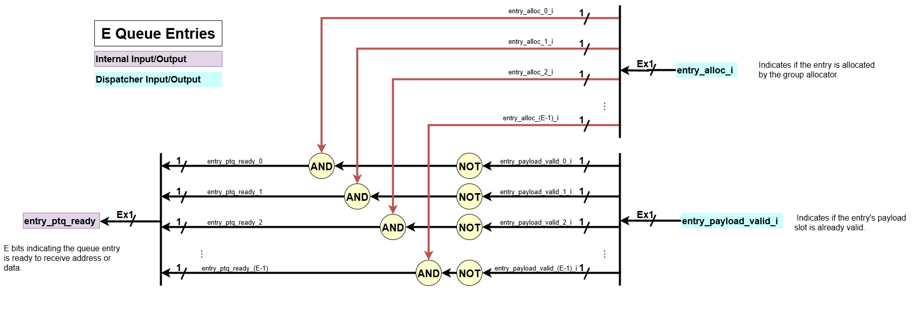
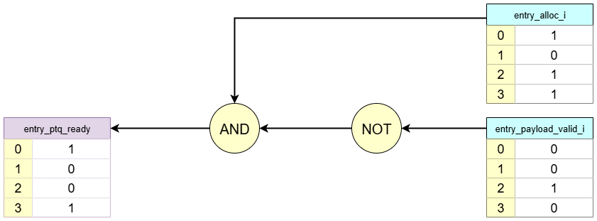
The Matching block is responsible for identifying which queue entries are actively waiting to receive an address or data payload.- Input:
entry_alloc_i: Indicates if the entry is allocated by the group allocator.entry_payload_valid_i: Indicates if the entry’s payload slot is already valid.
- Processing: For each queue entry, this block performs the check:
entry_alloc_i AND (NOT entry_payload_valid_i). An entry is considered waiting only if it has been allocated (entry_alloc_i = 1) but its payload slot is still empty (entry_payload_valid_i = 0) - Output:
entry_ptq_ready:N_ENTRIESbits indicating the queue entry is ready to receive address or data.
- Input:
-
Port Index Decoder
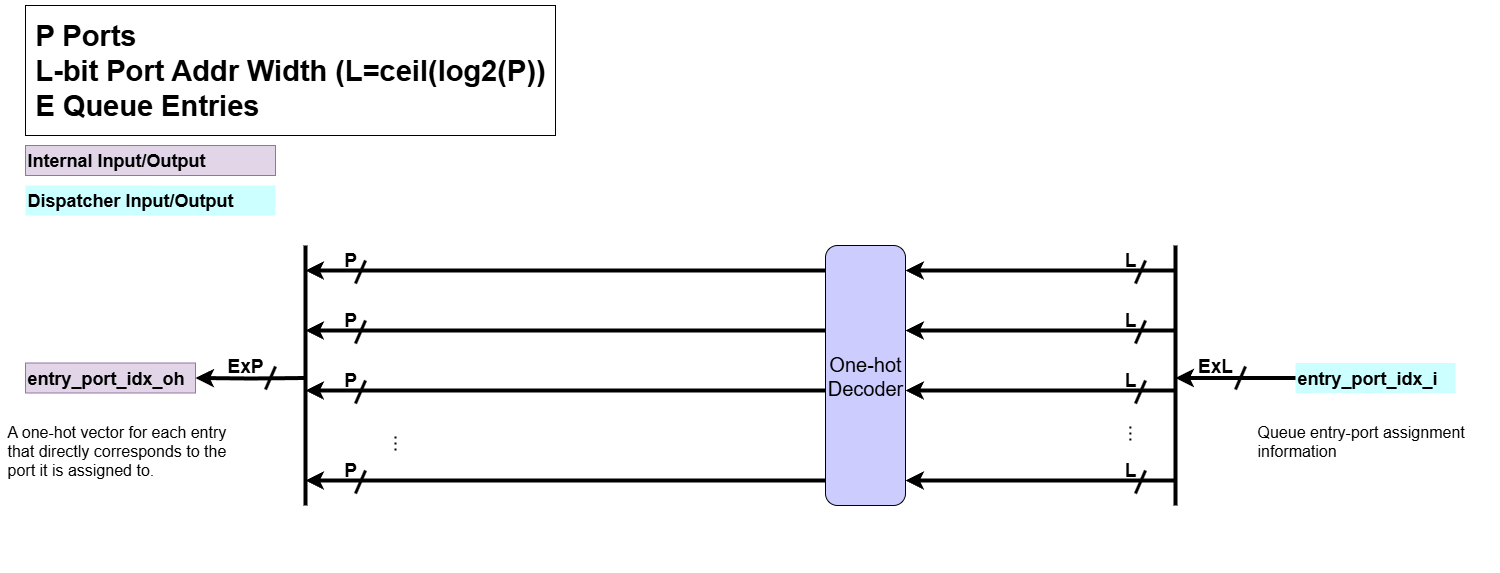
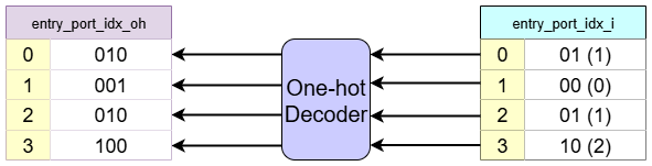
When the group allocator allocates a queue entry, it also assigns the queue entry to a specific port, storing this port assignment as an integer. The Port Index Decoder decodes the port assignment for each queue entry from an integer representation to a one-hot representation.- Input:
entry_port_idx_i: Queue entry-port assignment information
- Processing:
- It performs a integer-to-one-hot conversion on the port index associated with each entry. For example, if there are 3 ports, an integer index of
1 (01 in binary)would be converted to a one-hot vector of010.
- It performs a integer-to-one-hot conversion on the port index associated with each entry. For example, if there are 3 ports, an integer index of
- Output:
entry_port_idx_oh: A one-hot vector for each entry that directly corresponds to the port it is assigned to.
- Input:
-
Payload Mux
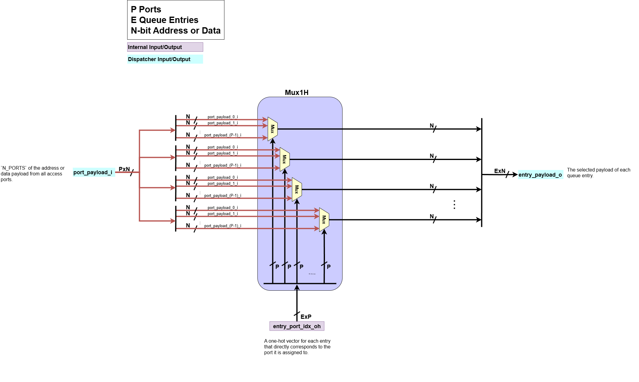
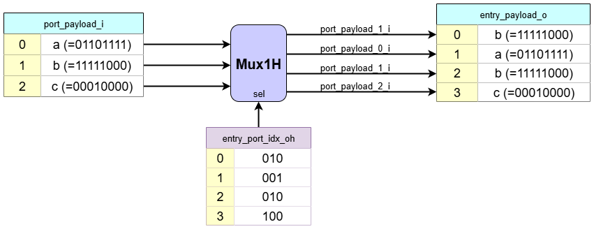
This block routes the address or data payload from the appropriate input port to the correct queue entries.- Input:
port_payload_i:N_PORTSof the address or data payload from all access ports.entry_port_idx_oh: The one-hot port assignment for each queue entry, used as the select signal.
- Processing: For each queue entry, a multiplexer
Mux1Huses the respectiveentry_port_idx_ohone-hot vector to select one payload fromport_payload_i. - Output:
entry_payload_o: The selected payload of each queue entry.
- Input:
-
Entry-Port Assignment Masking Logic
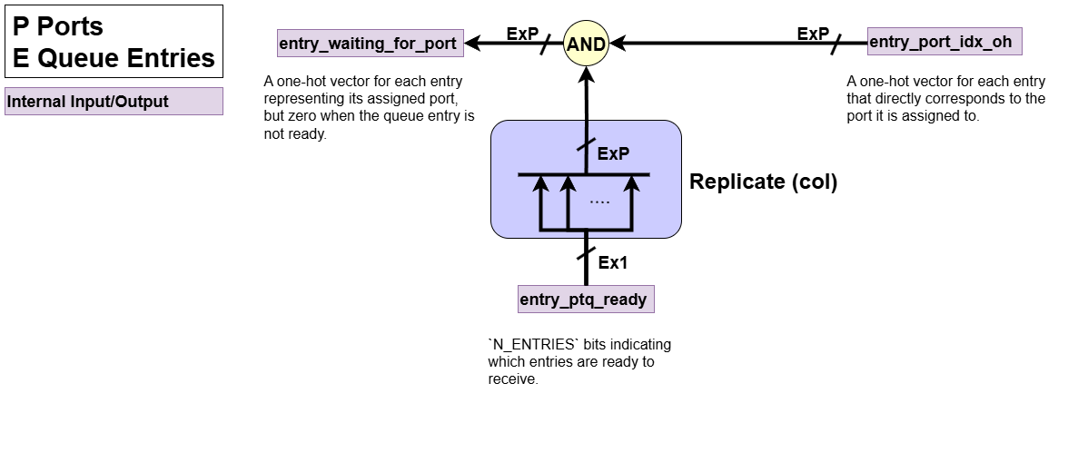
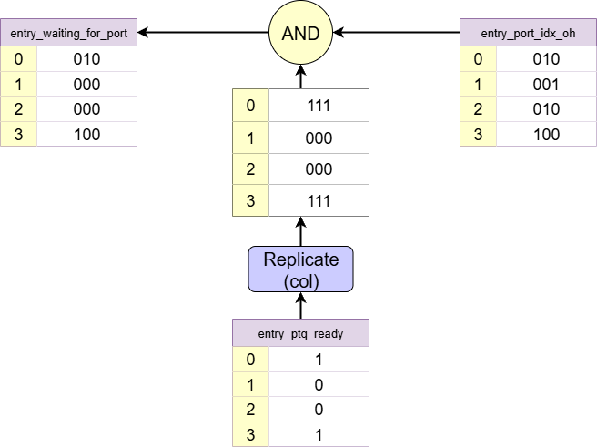
Each queue entry which is waiting for data, can only receive data from one port. This converts entry waiting from one-bit signal to a one-hot representation of the port it is waiting for the data from.
- Input:
entry_port_idx_oh: A one-hot vector for each entry representing its assigned port.entry_ptq_ready:N_ENTRIESbits indicating which entries are ready to receive.
- Processing: Performs a bitwise AND operation between each entry’s one-hot port assignment (
entry_port_idx_oh) and its readiness status (entry_ptq_ready). This masks out assignments for entries that are not waiting. - Output:
entry_waiting_for_port: A one-hot vector for each entry representing its assigned port, but zero when the queue entry is not ready.
- Input:
-
Handshake Logic
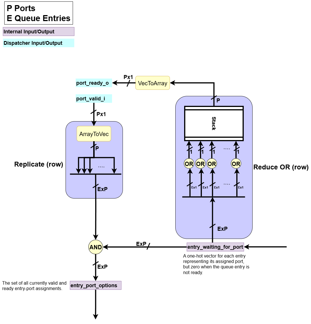
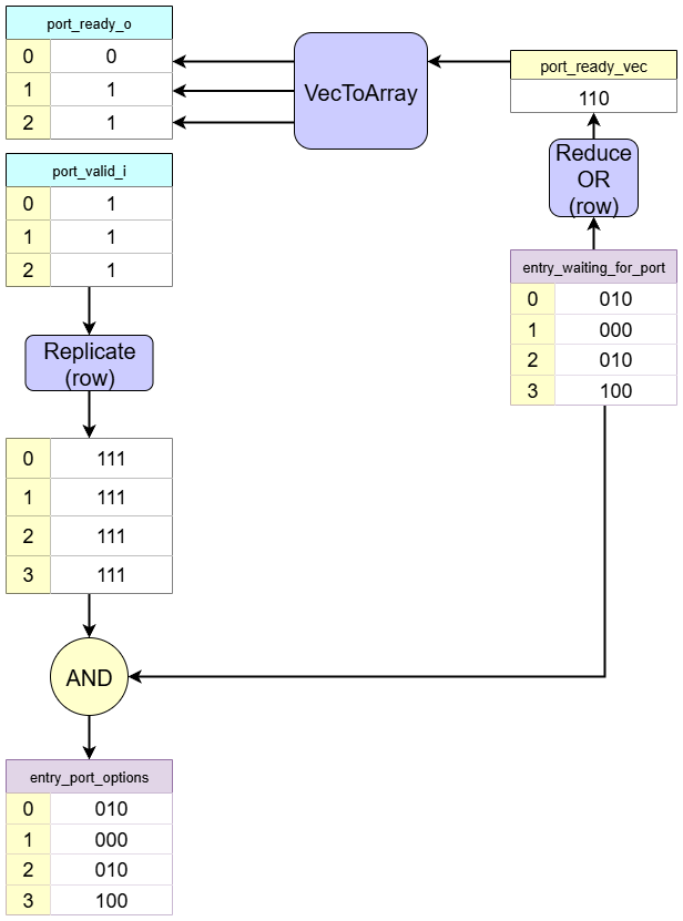
This block manages thevalid/readyhandshake protocol with the external access ports. It generates the outgoingport_ready_osignals and produces the final entry-port assignments that have completed a successful handshake (i.e. the internal request is ready and the external port is valid).- Input:
entry_waiting_for_port: A one-hot vector for each entry representing its assigned port, but zero when the queue entry is not ready.port_valid_i: The incoming port valid signals from each external port.
- Processing:
- Ready Generation: We determine if any queue entry is waiting for data from a specific port. If so, it asserts the
port_ready_osignal for that port to indicate it can accept data. - Handshake: It then uses the external
port_valid_isignals to mask out entries inentry_waiting_for_portif the respective port is not valid. It usesVecToArrayoperations to convertP-bitvector intoP1-bit signals.
- Ready Generation: We determine if any queue entry is waiting for data from a specific port. If so, it asserts the
- Output:
port_ready_o: The outgoing ready signal to each external port.entry_port_options: Represents the set of handshaked entry-port assignments. This signal indicates a successful handshake and is sent to the Arbitration Logic to select the oldest one.
- Input:
-
Arbitration Logic
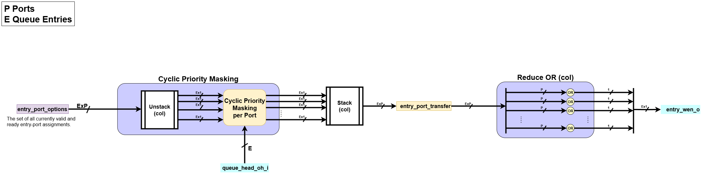
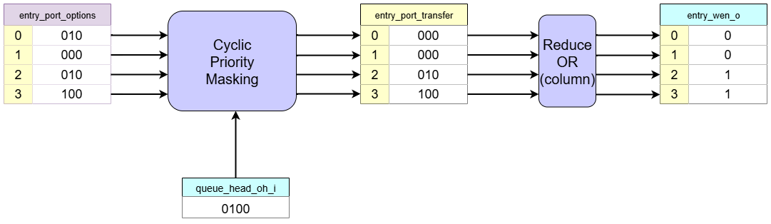
The core decision making block of the dispatcher. When multiple handshaked entry-port assignments are ready to be written in the same cycle, it chooses the oldest queue entry among the valid ones for each port.- Input:
entry_port_options: The set of all currently valid and ready entry-port assignments.queue_head_oh_i: The queue’s one-hot head vector.
- Processing: It uses a
CyclicPriorityMaskingalgorithm. This ensures that among all candidates for each port, the one corresponding to the oldest entry in the queue is granted for the current clock cycle. - Output:
entry_wen_osignal, which acts as the enable for the queue entry. This signal ultimately causes the queue’sentry_payload_validsignal to go high via logic outside of the dispatcher.
- Input:
3. Dataflow Walkthrough
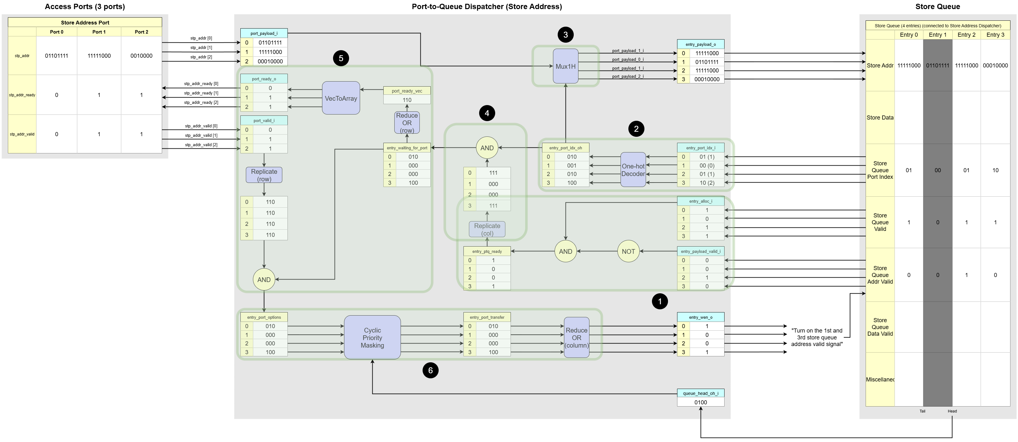
Example of Store Address Port-to-Queue Dispatcher (3 Store Ports, 4 Store Queue Entries)
-
Matching: Identifying which queue slots are empty
The first job of this block is to determine which entries in the store queue are waiting for a store address.Based on the example diagram:
- Entry 1 is darkened to indicate that it has not been allocated by the Group Allocator. Its
Store Queue Validsignal (equivalent toentry_alloc_i) is0. - Entries 0, 2, and 3 have been allocated, so their
entry_alloc_isignal are1. However, among these, Entry 2 already has a valid address (Store Queue Addr Valid = 1). - Therefore, only
Entries 0 and 3are actively waiting for their store address, as they are allocated but theirStore Queue Addr Validbit is still0.
This logic is captured by the expression
entry_ptq_ready = entry_alloc_i AND (NOT entry_payload_valid_i), which creates a list of entries that need attention from the dispatcher. - Entry 1 is darkened to indicate that it has not been allocated by the Group Allocator. Its
-
Port Index Decoder: Queue entries port assignment in one-hot format
This block’s circuit is to decode an integer index assigned to each queue entry into a one-hot format.Based on the example diagram:
- The
Store Queueshows thatEntry 0is assigned toPort 1,Entry 1toPort 0,Entry 2toPort 1andEntry 3toPort 2. - The
Port Index Decodertakes these integer indices (0,1,2) as input which are (00,01,02in binary respectively). - It processes them and generates a corresponding one-hot vector for each entry. Since there are three access ports, the vector are three bits wide:
Entry 0 (Port 1):010Entry 1 (Port 0):000Entry 2 (Port 1):010Entry 3 (Port 2):100
The output of this block,
N_ENTRIESof one-hot vectors, is a crucial input for thePayload Mux, where it acts as the select signal to choose the data from the correct port. - The
-
Payload Mux: Routing the correct address
Based on the example diagram:
- The
Access Portstable shows the current address payloads being presented by each port:Port 0:01101111Port 1:11111000Port 2:00100000
- The
Port Index Decoderhas already determined the port assignments for each entry - The
Payload Muxuses these assignments to perform the selection:Entry 0:11111000(Address fromPort 1)Entry 1:01101111(Address fromPort 0)Entry 2:11111000(Address fromPort 1)Entry 3:00100000(Address fromPort 2)
The output of this block,
entry_payload_ois logically committed to the queue only when theArbitration Logicasserts theentry_wen_osignal for that specific entry. - The
-
Entry-Port Assignment Masking Logic
Based on the example diagram:
-
entry_ptq_ready:Entry 0:1(Entry 0 is waiting) ->111Entry 1:0(Entry 1 is not waiting) ->000Entry 2:0(Entry 2 is not waiting) ->000Entry 3:1(Entry 3 is waiting) ->111
-
entry_port_idx_oh:Entry 0:010(Port 1)Entry 1:000(Port 0)Entry 2:010(Port 1)Entry 3:100(Port 2)
-
Bitwise AND operation
Entry 0:111AND010=010Entry 1:000AND000=000Entry 2:000AND010=000Entry 3:111AND100=100
entry_waiting_for_port: It now only contains one-hot vectors for entries that are both allocated and waiting for a payload.
-
-
Handshake Logic: Managing port readiness and masking the port assigned with invalid ports
This block is responsible for thevalid/readyhandshake protocol with theAccess Ports. It performs two functions: providing back-pressure to the ports and identifying all currently active memory requests for the arbiter. The value ofentry_waiting_for_portis different from the previous step for the robustness of the example.Based on the example diagram:
- Back-pressure control: First, the block determines which ports are
ready.- From the
Entry-Port Assignment Masking Logicblock, we know thatEntry 0,Entry 2, andEntry 3are waiting for an address fromPort 1andPort 2. - Therefore, it asserts
port_ready_oto1for bothPort 1andPort 2. - No entry is waiting for
Port 0, so its ready signal is0.
- From the
- Active request filtering: The block checks which ports are handshaked. The
Access Portstable showsport_valid_iis1for allPort 0,Port 1andPort 2. Since the waiting entries fromentry_waiting_for_port(Entry 0,Entry 2, andEntry 3) correspond to the valid ports (Port 1andPort 2), both are considered active and are passed to theArbitration Logic.
- Back-pressure control: First, the block determines which ports are
-
Arbitration Logic: Selecting the oldest active entry
This block is responsible for selecting the oldest active memory request for each port and generating the write enable signal for such requests.Based on the example diagram:
- The
Handshake Logichas identified three active requests: one forEntry 0fromPort 1, another forEntry 2fromPort 1, and the other forEntry 3fromPort 2. - The CyclicPriorityMasking algorithm operates independently on each port’s request list.
- For
Port 2, the only active request is fromEntry 3(0001, the left column ofentry_port_options). With no other competitors for this port,Entry 3is selected as the oldest forPort 2. - For
Port 1, the active requests are fromEntry 0andEntry 2(0101, the middle column ofentry_port_options). Since the head of the queue is atEntry 2, it is the oldest entry.Entry 0is masked out byCyclicPriorityMasking.
- For
As a result, the
entry_wen_osignal is asserted for bothEntry 0andEntry 3, allowing two writes to proceed in parallel in the same clock cycle. - The
Queue-to-Port Dispatcher
How loaded data get back to where it belongs.
1. Overview and Purpose
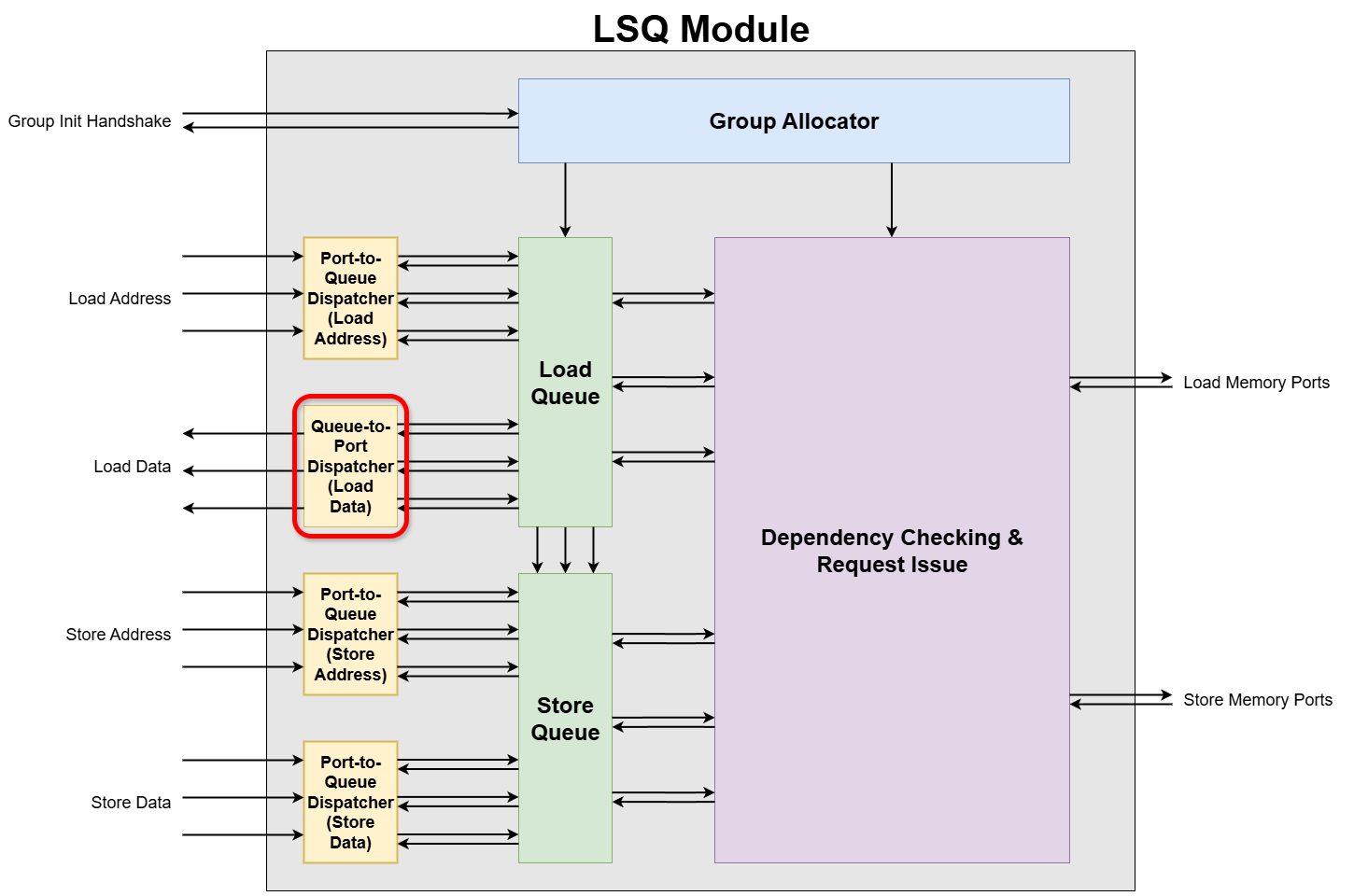
The Queue-to-Port Dispatcher is the counterpart to the Port-to-Queue Dispatcher. Its responsibility is to route payloads—primarily data loaded from memory—from the queue entries back to the correct access ports of the dataflow circuit.
While the LSQ can process memory requests out-of-order, the results for a specific access port must be returned in program order to maintain the correctness. This module ensures that this order is respected for each port.
The primary instance of this module is the Load Data Port Dispatcher, which sends loaded data back to the circuit. An optional second instance, the Store Backward Port Dispatcher, can be used to send store completion acknowledgements back to the circuit.
2. Queue-to-Port Dispatcher Internal Blocks
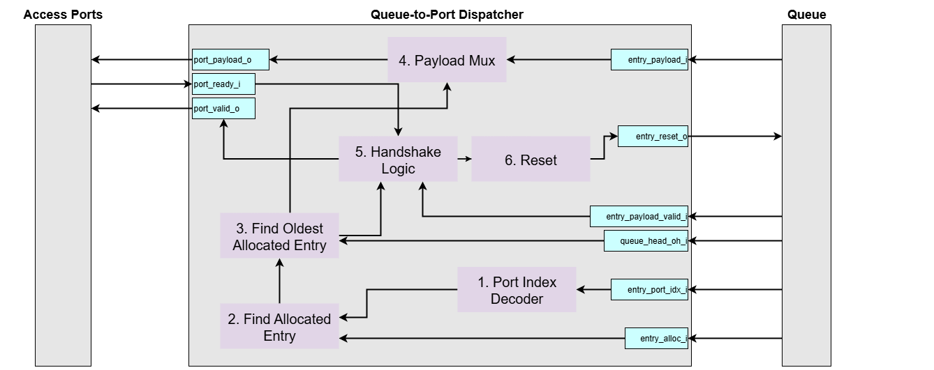
Let’s assume the following generic parameters for dimensionality:
N_PORTS: The total number of ports.N_ENTRIES: The total number of entries in the queue.PAYLOAD_WIDTH: The bit-width of the payload (e.g., 8 bits).PORT_IDX_WIDTH: The bit-width required to index a port (e.g.,ceil(log2(N_PORTS))).
Signal Naming and Dimensionality:
This module is generated from a higher-level description (e.g., in Python), which results in a specific convention for signal naming in the final VHDL code. It’s important to understand this convention when interpreting diagrams and signal tables.
-
Generation Pattern: A signal that is conceptually an array in the source code (e.g.,
port_payload_o) is “unrolled” into multiple, distinct signals in the VHDL entity. The generated VHDL signals are indexed with a suffix, such asport_payload_{p}_o, where{p}is the port index. -
Interpreting Diagrams: If a diagram or conceptual description uses a base name without an index (e.g.,
port_payload_o), it represents a collection of signals. The actual dimension is expanded based on the context:- Port-related signals (like
port_payload_o) are expanded by the number of ports (N_PORTS). - Entry-related signals (like
entry_alloc_o) are expanded by the number of queue entries (N_ENTRIES).
- Port-related signals (like
Port Interface Signals
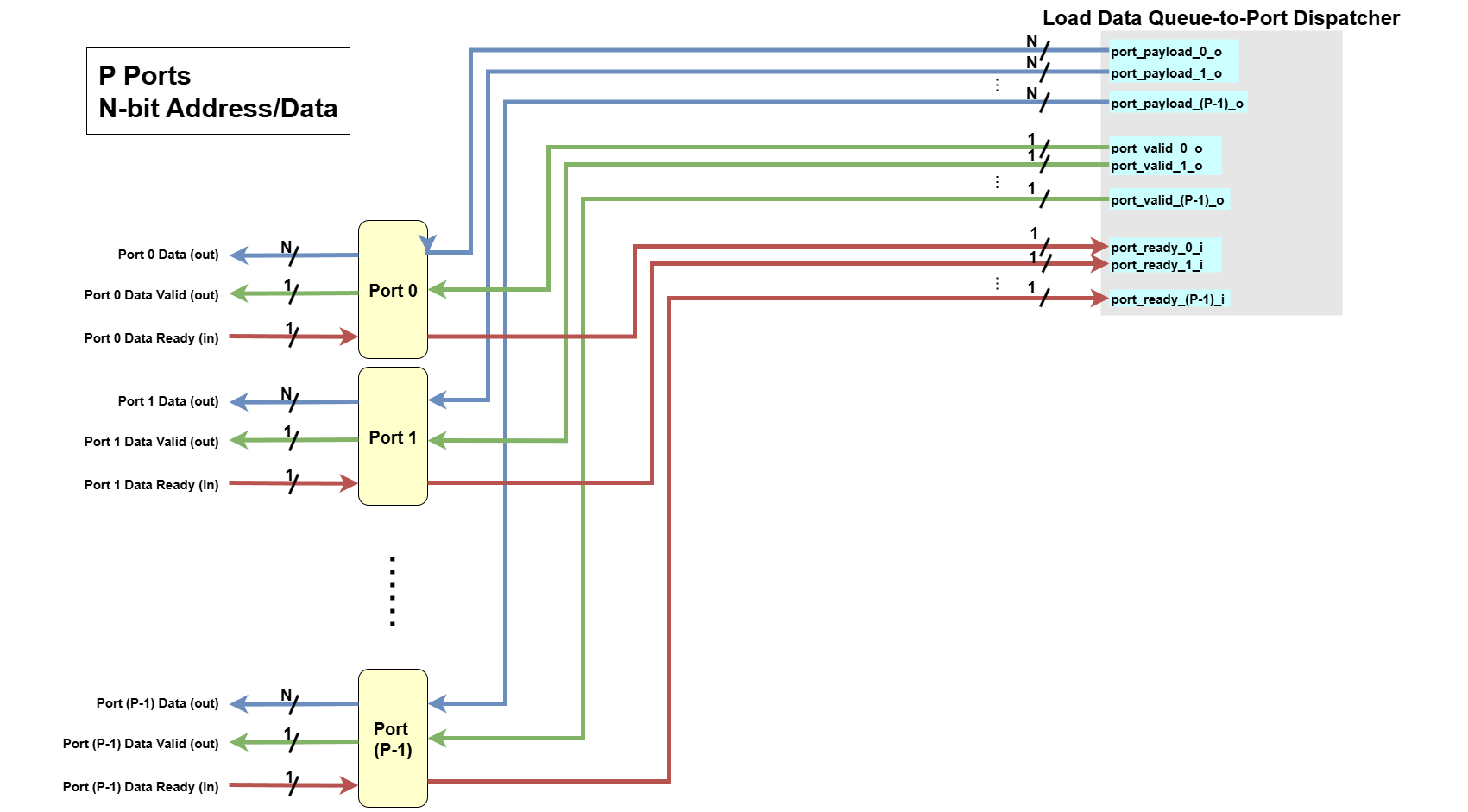
These signals are used for communication between the external modules and the dispatcher’s ports.
| Python Variable Name | VHDL Signal Name | Direction | Dimensionality | Description |
|---|---|---|---|---|
| Inputs | ||||
port_ready_i | port_ready_{p}_i | Input | std_logic | Ready flag from port p. port_ready_{p}_i is high when the external circuit is ready to receive data. |
| Outputs | ||||
port_payload_o | port_payload_{p}_o | Output | std_logic_vector(PAYLOAD_WIDTH-1:0) | Data payload sent to port p. |
port_valid_o | port_valid_{p}_o | Output | std_logic | Valid flag for port p. Asserted to indicate that port_payload_{p}_o contains valid data. |
Queue Interface Signals
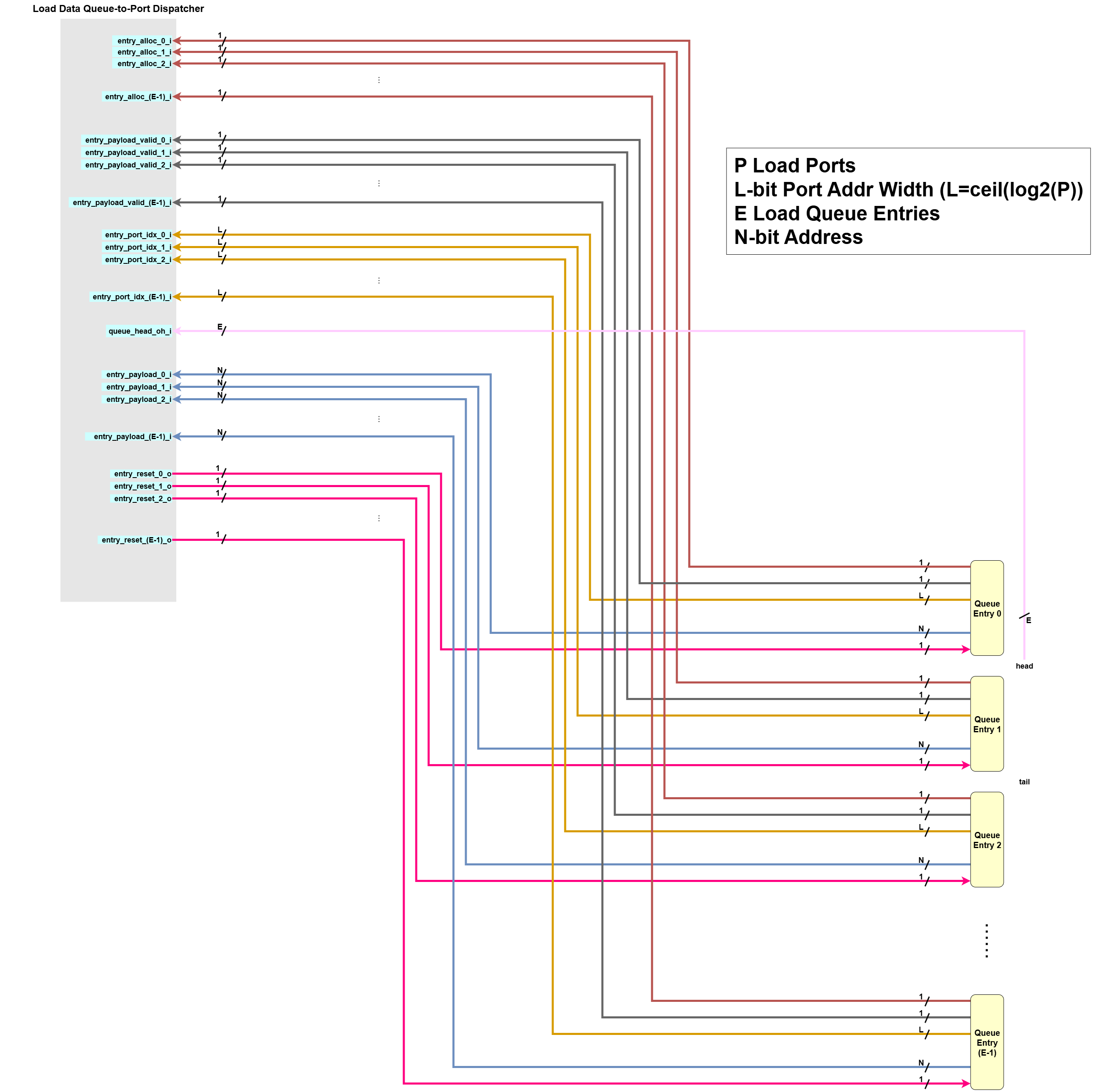
These signals handle the interaction between the dispatcher logic and the internal queue entries.
| Python Variable Name | VHDL Signal Name | Direction | Dimensionality | Description |
|---|---|---|---|---|
| Inputs | ||||
entry_alloc_i | entry_alloc_{e}_i | Input | std_logic | Is queue entry e logically allocated? |
entry_payload_valid_i | entry_payload_valid_{e}_i | Input | std_logic | Is the result data in entry e valid and ready to be sent? |
entry_port_idx_i | entry_port_idx_{e}_i | Input | std_logic_vector(PORT_IDX_WIDTH-1:0) | Indicates to which port entry e is assigned. |
entry_payload_i | entry_payload_{e}_i | Input | std_logic_vector(PAYLOAD_WIDTH-1:0) | The data stored in queue entry e. |
queue_head_oh_i | queue_head_oh_i | Input | std_logic_vector(N_ENTRIES-1:0) | One-hot vector indicating the head entry in the queue. |
| Outputs | ||||
entry_reset_o | entry_reset_{e}_o | Output | std_logic | Reset signal for an entry. entry_reset_{e}_o is asserted to deallocate entry e after its data has been successfully sent. |
The Queue-to-Port Dispatcher has the following core responsibilities (with 3-port, 4-entry load data dispatcher example):
-
Port Index Decoder

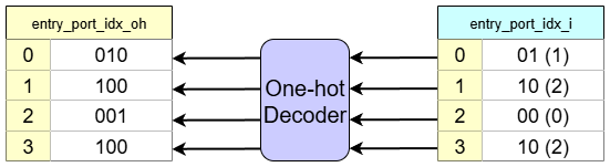
When the group allocator allocates a queue entry, it also assigns the queue entry to a specific port, storing this port assignment as an integer. The Port Index Decoder decodes the port assignment for each queue entry from an integer representation to a one-hot representation.- Input:
entry_port_idx_i: Queue entry-port assignment information
- Processing:
- It performs a integer-to-one-hot conversion on the port index associated with each entry. For example, if there are 3 ports, an integer index of
1 (01 in binary)would be converted to a one-hot vector of010.
- It performs a integer-to-one-hot conversion on the port index associated with each entry. For example, if there are 3 ports, an integer index of
- Output:
entry_port_idx_oh: A one-hot vector for each entry that directly corresponds to the port it is assigned to.
- Input:
-
Find Allocated Entry
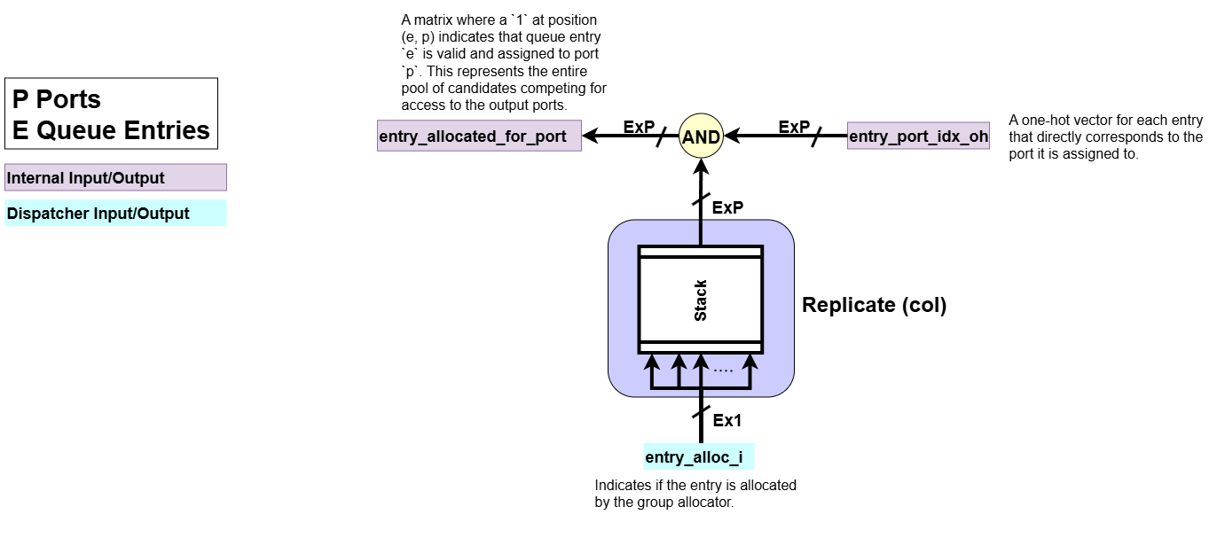
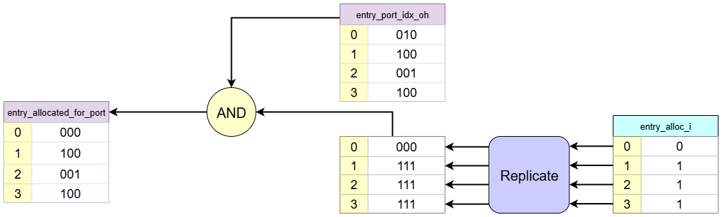
This block identifies which entries in the queue are currently allocated (entry_alloc_{e}_i=1), meaning whether each entry is allocated by the group allocator or not.- Input:
entry_alloc_i: Indicates if the entry is allocated by the group allocator.entry_port_idx_oh: A one-hot vector for each entry that directly corresponds to the port it is assigned to.
- Processing:
- For each queue entry
e, this block performs the check:entry_alloc_i AND entry_port_idx_oh. - If an entry is not allocated (i.e., not allocated by the group allocator,
entry_alloc_{e}_i = 0), its port assignment is masked, resulting in a zero vector. - If the entry is allocated (i.e., allocated,
entry_alloc_{e}_i = 1), its one-hot port assignment is passed through unchanged.
- For each queue entry
- Output:
entry_allocated_per_port: The resulting matrix where a1at position(e,p)indicates that entryeis allocated and assigned to portp. This matrix represents all potential candidates for sending data and is fed into the arbitration logicCyclicPriorityMaskingto determine which entry gets to send its data first for each port.
- Input:
-
Find Oldest Allocated Entry
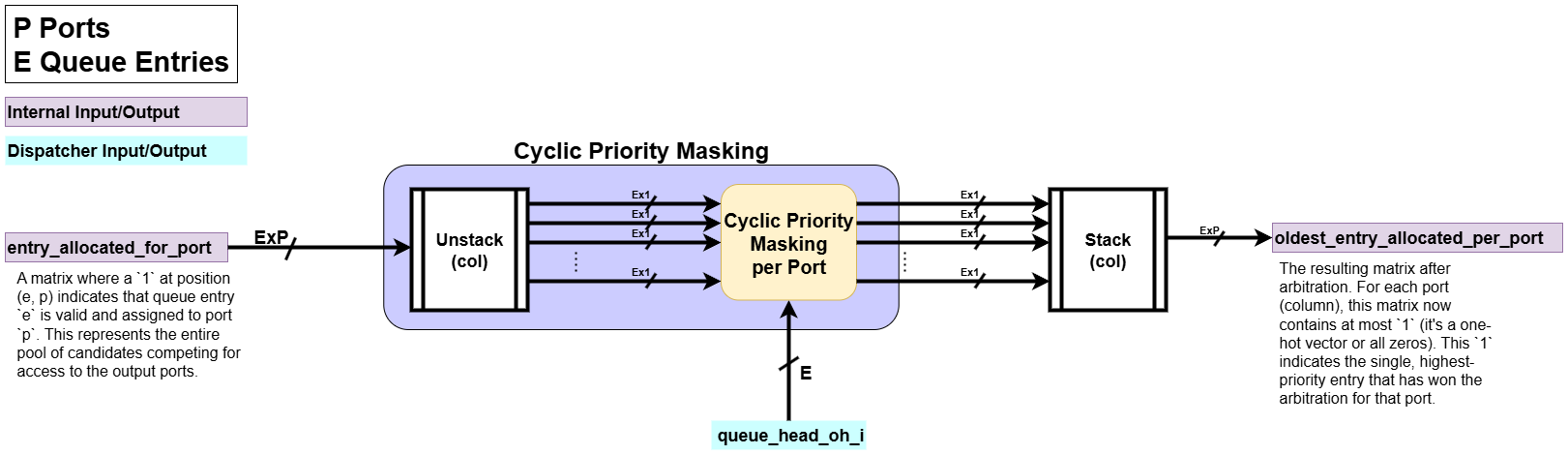
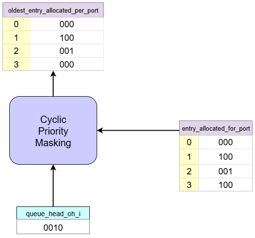
This is the core Arbitration Logic of the dispatcher. It takes all potential requests and selects a single “oldest” for each port based on priority.- Input:
entry_allocated_per_port: A matrix where a1at position (e, p) indicates that queue entryeis allocated and assigned to portp. This represents the entire pool of candidates competing for access to the output ports.queue_head_oh_i: The queue’s one-hot head vector, which represents the priority (i.e., the oldest entry) for the current cycle.
- Processing:
- It uses a CyclicPriorityMasking algorithm, which operates on each port (column of
entry_allocated_per_port). - This ensures that among all candidates for each port, the one corresponding to the oldest entry in the queue is granted for the current clock cycle.
- It uses a CyclicPriorityMasking algorithm, which operates on each port (column of
- Output:
oldest_entry_allocated_per_port: The resulting matrix after arbitration. For each port (column), this matrix now contains at most1(it’s a one-hot vector or all zeros). This1indicates the single, highest-priority entry that has won the arbitration for that port.
- Input:
-
Payload Mux
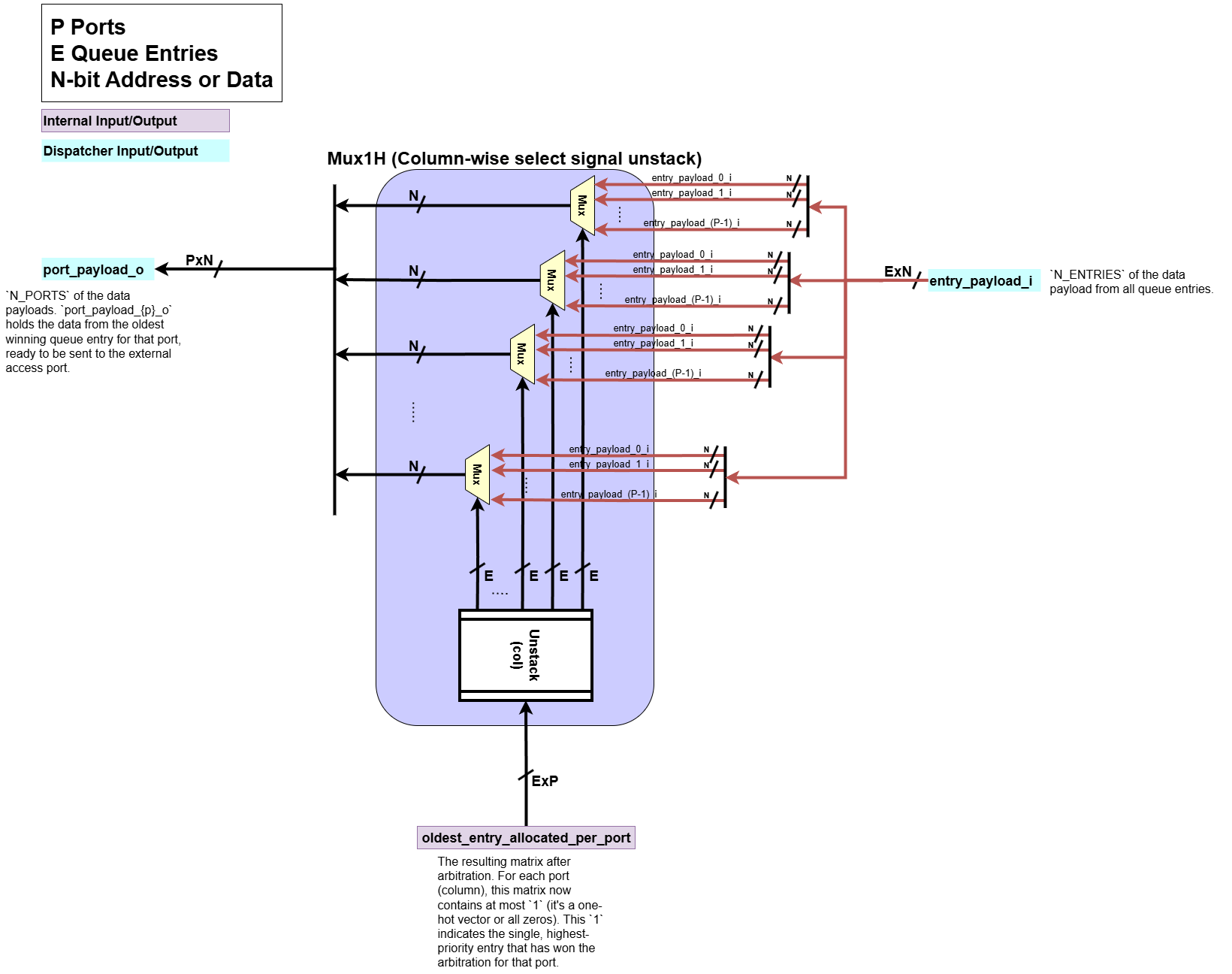
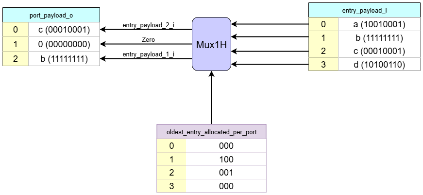
For each access port, this block routes the payload from the oldest queue entry to the correct output port.- Input:
entry_payload_i:N_ENTRIESof the data payload from all queue entries.oldest_entry_allocated_per_port: The arbitrated selection matrix from the Find Oldest Allocated Entry block. For each port (column), this matrix contains at most a single1, which identifies the oldest entry for that port.
- Processing:
- For each output port
p, a one-hot multiplexer (Mux1H) uses thep-th column of theoldest_entry_allocated_per_portmatrix as its select signal. - This operation selects the data payload from the single oldest entry out of the entire
entry_payload_iand routes it to the corresponding output port.
- For each output port
- Output:
port_payload_o:N_PORTSof the data payloads.port_payload_{p}_oholds the data from the oldest queue entry for that port, ready to be sent to the external access port.
- Input:
-
Handshake Logic
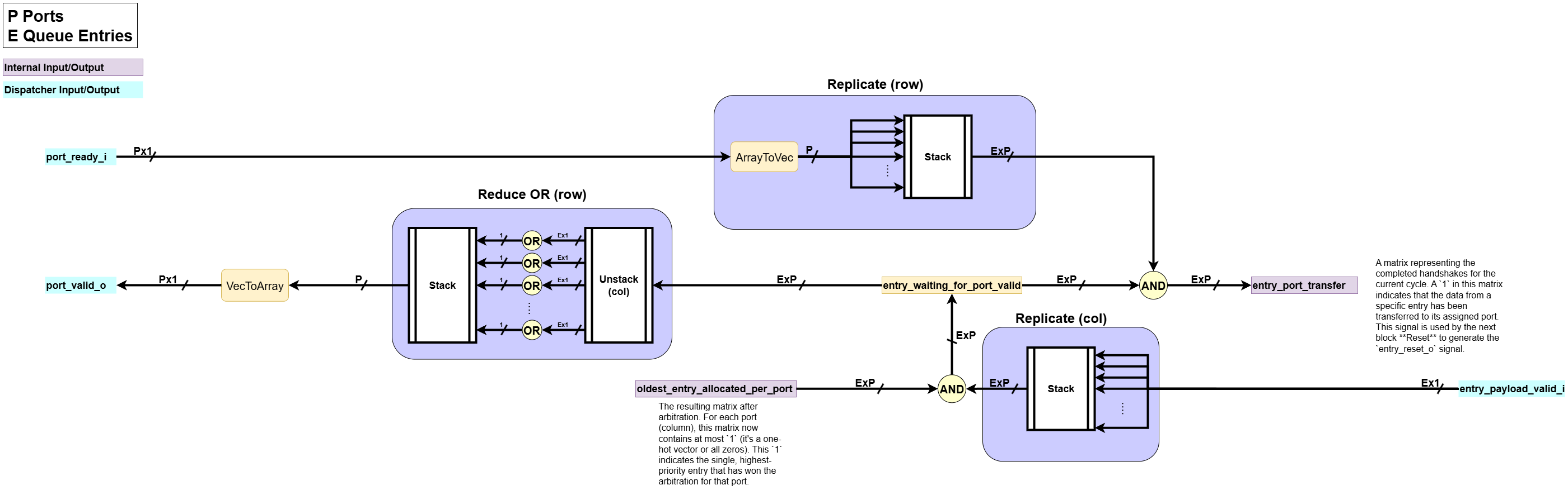
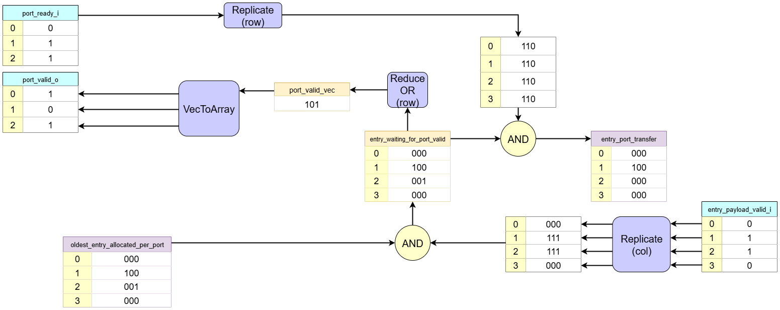
This block manages thevalid/readyhandshake with the external access ports. It checks that the oldest entry’s data from the cyclic priority masking is valid and that the receiving port is ready, then generates a signal indicating that it is transferred.- Input:
port_ready_i:N_PORTSof the ready signals from the external access ports.port_ready_{p}_iis high when portpcan accept data.entry_payload_valid_i: Each of theN_ENTRIESindicates whether the data slot of queue entryeis valid and ready to be sent.oldest_entry_allocated_per_port: The arbitrated selection matrix from the Find Oldest Allocated Entry block, indicating at most the single oldest entry for each port.
- Processing:
- Check the Oldest’s Data Validity: First, the block verifies if the data in the oldest entry is actually ready. It masks the
oldest_entry_allocated_per_portmatrix with theentry_payload_valid_i. If the oldest entry for a port doesn’t have valid data, it is nullified for this cycle. The result isentry_waiting_for_port_valid. - Generate
port_valid_o: The result of the masking from the previous step is then reduced (OR-reduction) for each port. If any entry in a column is still valid, it means a oldest entry with valid data exists for that port, and the correspondingport_valid_osignal is asserted high. - Perform Handshake: Next, it determines if a successful handshake occurs. For each port
p, a handshake is successful if the dispatcher has valid data to send (port_valid_{p}_ois high) AND the external port is ready to receive it (port_ready_{p}_iis high).
- Check the Oldest’s Data Validity: First, the block verifies if the data in the oldest entry is actually ready. It masks the
- Output:
port_valid_o: The final valid signal sent to each external access port, indicating that valid data is available on theport_payload_obus.entry_port_transfer: A matrix representing the completed handshakes for the current cycle. A1in this matrix indicates that the data from a specific entry has been transferred to its assigned port. This signal is used by the next block Reset to generate theentry_reset_osignal.
- Input:
-
Reset
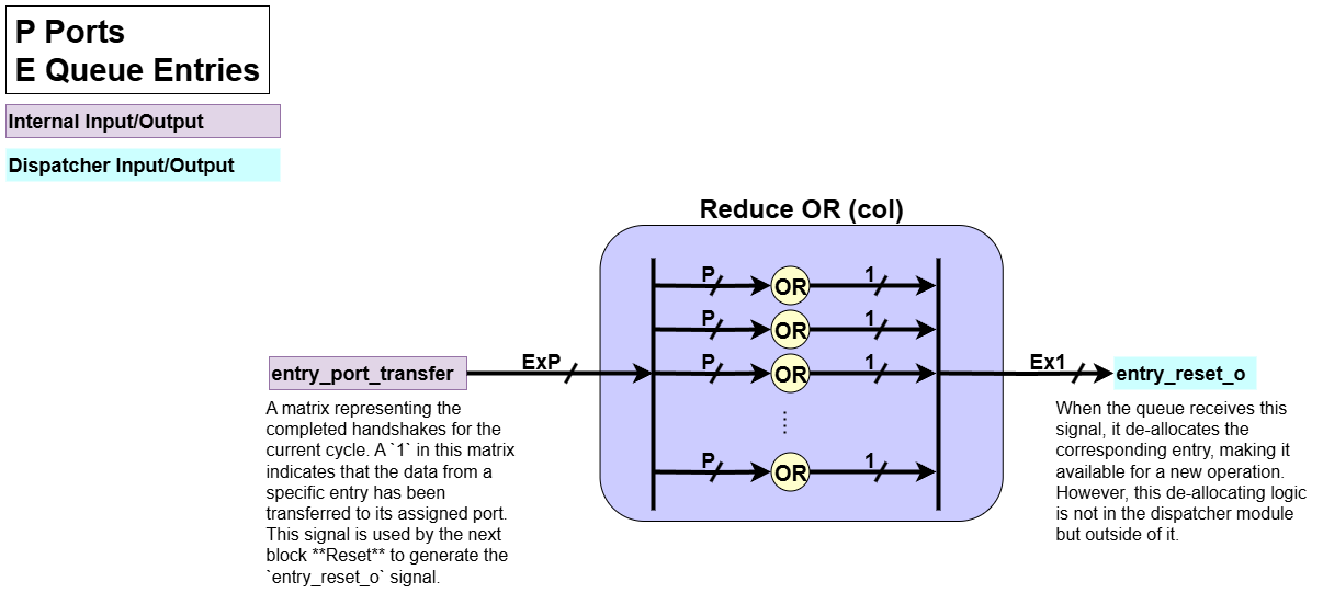
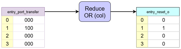
This block is responsible for clearing a queue entry after its payload has been successfully dispatched.- Input:
entry_port_transfer: A matrix representing the completed handshakes for the current cycle. A1in this matrix indicates that the data from a specific entry has been transferred to its assigned port.
- Processing:
- Checks each entry (row) of
entry_port_transferwhether it has1in a given rowe. It means that entryesent its data to some port. - Performs an OR operation across each row.
- Checks each entry (row) of
- Output:
entry_reset_o: When the queue receives this signal, it de-allocates the corresponding entry, making it available for a new operation. However, this de-allocating logic is not in the dispatcher module but outside of it.
- Input:
3. Dataflow Walkthrough
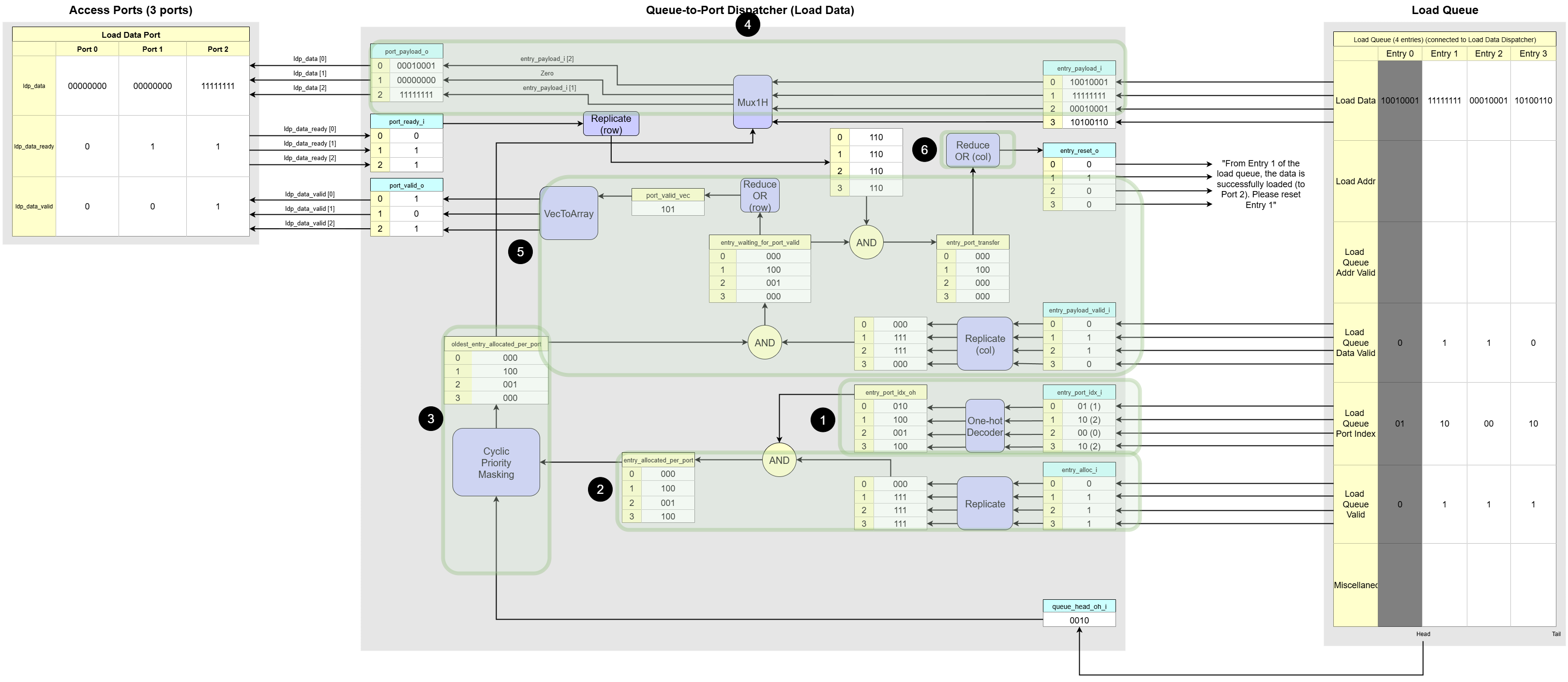
-
Initial state:
- Port Assignments:
- Entry 0 -> Port 1
- Entry 1 -> Port 2
- Entry 2 -> Port 0
- Entry 3 -> Port 2
- Queue Head: At
Entry 1. entry_alloc_i:[0, 1, 1, 1](Entries 1, 2, 3 are allocated).entry_payload_valid_i:[0, 1, 1, 0](Entries 1, 2 have valid data).port_ready_i:[0, 1, 1](Ports 1 and 2 are ready, Port 0 is not).
- Port Assignments:
-
Port Index Decoder
This block translates the integer port index assigned to each queue entry into a one-hot vector.
Based on the example diagram:-
The
Port Index Decoderconverts these integer port indices into 3-bit one-hot vectors:Entry 0 (Port 1):010Entry 1 (Port 2):100Entry 2 (Port 0):001Entry 3 (Port 2):100
-
This result is saved in
entry_port_idx_ohentry_port_idx_oh P2 P1 P0 E0: [ 0, 1, 0 ] E1: [ 1, 0, 0 ] E2: [ 0, 0, 1 ] E3: [ 1, 0, 0 ]
-
-
Find Allocated Entry
This block identifies all queue entries that are candidates for dispatching. Based on the example diagram:- The
entry_alloc_ivector is[0, 1, 1, 1]. Therefore, Entries 1, 2, and 3 are the potential candidates to send their data out. - The logic then combines this allocation information with the one-hot decoded port index for each entry (
entry_port_idx_ohfrom thePort Index Decoder). An entry’s one-hot port information is passed through only if its correspondingentry_alloc_ibit is1. - If an entry is not allocated (like
Entry 0), its output for this stage is zeroed out (000). - The result is the
entry_allocated_per_portmatrix, which represents the initial list of all allocated queue entries and their target ports. This matrix is then sent to theFind Oldest Allocated Entryblock for arbitration.
- The
-
Find Oldest Allocated Entry
This is the core Arbitration Logic. It selects a single “oldest” for each port from the list of allocated candidates, based on priority.
Based on the example diagram:- The queue head is at
Entry 1, establishing a priority order of1 -> 2 -> 3 -> 0. Port 0: The only allocated candidate isEntry 2. It is the oldest for Port 0.Port 1: There are no valid candidates assigned to this port.Port 2: The valid candidates areEntry 1andEntry 3. According to the priority order,Entry 1is the oldest forPort 2.- The output indicates that
Entry 2is the oldest forPort 0, andEntry 1is the oldest forPort 2. - The result is
oldest_entry_allocated_per_port
- The queue head is at
-
Payload Mux
This block routes the data from the oldest entries to the correct output ports.
Based on the example diagram:-
For
port_payload_o[0], it selects the data from the oldest entry ofPort 0,Entry 2. -
For
port_payload_o[2], it selects the data from the oldest entry ofPort 2,Entry 1. -
For
Port 1,0is assigned. -
The result is
port_payload_oport_payload_o P0: entry_payload_i [2] = 00010001 P1: Zero = 00000000 P2: entry_payload_i [1] = 11111111
-
-
Handshake Logic
This block manages the final stage of the dispatch handshake. It first generates theport_valid_osignals by checking if the oldest one from arbitration have valid data to send. It then confirms which of these can complete a successful handshake.
Based on the example diagram:-
First, the logic checks the
entry_payload_valid_ivector, which is[0, 1, 1, 0]. This indicates that among the oldest queue entries, data is valid and ready to be sent fromEntry 1andEntry 2. -
For the
Port 0oldest (Entry 2), itsentry_payload_valid_iis1. The logic assertsport_valid_o[0]to1. -
For the
Port 2oldest (Entry 1), itsentry_payload_valid_iis1. The logic assertsport_valid_o[2]to1. -
Next, the logic checks incoming
port_ready_isignals from the access ports, which are[0, 1, 1]. This means thatPort 1andPort 2are ready, butPort 0is not. A final handshake is successful only if the dispatcher has valid data to sendANDthe port is ready to receive. Theentry_port_transfermatrix shows this final result:entry_port_transfer P2 P1 P0 E0: [ 0, 0, 0 ]` E1: [ 1, 0, 0 ] // Handshake succeeds (valid=1, ready=1) E2: [ 0, 0, 0 ] // Handshake fails (valid=1, ready=0) E3: [ 0, 0, 0 ] -
This means: “Even though the queue is sending valid data to Port 0 and Port 2, only the handshake with Port 2 is successful because only Port 2 is ready to receive data.”
-
-
Reset
This block is responsible for generating theentry_reset_osignal, which clears an entry in the queue after its data has been successfully dispatched. A successful dispatch requires a completevalid/readyhandshake.
Based on the initial state:- The Reset block asserts
entry_reset_oonly for the entry corresponding to the successful handshake, which isEntry 1. The message in the diagram confirms this: “From Entry 1 of the load queue, the data is sent to Port 2. Please reset Entry 1”.
- The Reset block asserts
Adding Spec Tags to Speculative Region
The spec tag, required for speculation, is added as an extra signal to operand/result types (e.g., ChannelType or ControlType).
Type verification ensures that circuits include extra signals like the spec tag, but it does not automatically update or infer them. Therefore, we need an explicit algorithm to do it.
This document outlines the algorithm for adding spec tags to operand/result types within a speculative region.
Implementation
The algorithm uses depth-first search (DFS) starting from the speculator, adding spec tags to each traversed operand. It performs both upstream and downstream traversal.
Consider the following example (omitting the input to the speculator for simplicity):
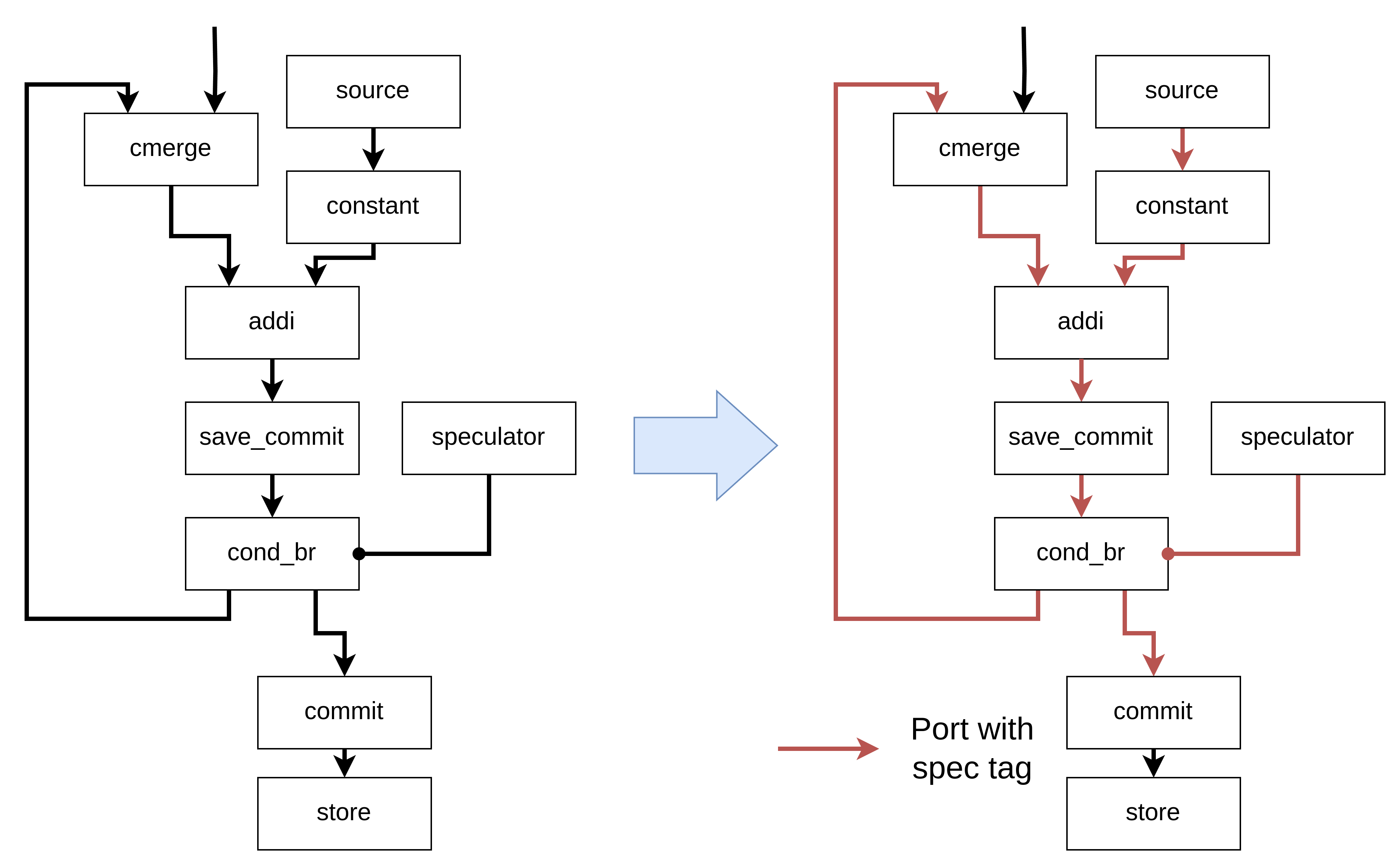
The algorithm follows these steps:
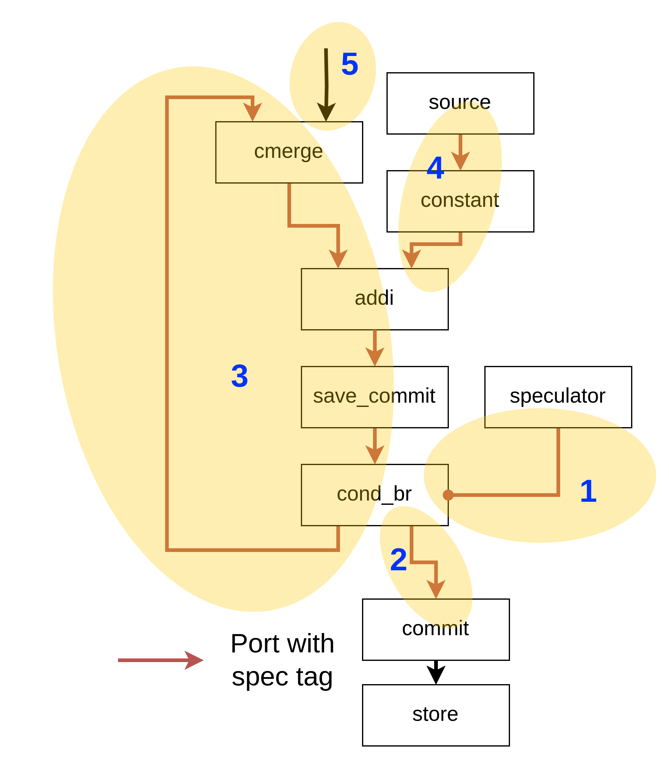
-
Start DFS from the speculator, first reaching
cond_br. -
Downstream traversal stops at the commit unit.
-
Another downstream traversal reaches
cmerge,addi,save_commit, and eventuallycond_bragain. Sincecond_bris already visited, traversal stops there. -
Upstream traversal is applied from
additoconstantandsource, ensuring that spec tags are added to these operands, asaddienforces consistent extra signals across all their inputs and outputs. -
Upstream traversal is skipped for
cmergeandmux, since some of their operands originate outside the speculative region. All internal edges are covered by downstream traversal.
Special Cases
The following edges are skipped:
- Edges inside the commit and save-commit control networks
- Edges leading to memory controllers
When the traversal reaches the relevant units (e.g., save_commit, commit, speculating_branch, or load), it doesn’t proceed to these edges but continues with the rest of the traversal.
Commit Unit Placement Algorithm
The placement of commit units is determined by a Depth-First Search (DFS) starting from the Speculator. When the traversal reaches specific operations, it stops the traversal and places a commit unit in front of these operations:
- StoreOp
- EndOp
- MemoryControllerOp
Note that commit units are not placed for LoadOp.
Commit Units for MemoryControllerOp
MemoryControllerOp is a bit complex, as we want to place commit units for some operands but not for others. Here’s how we place them:
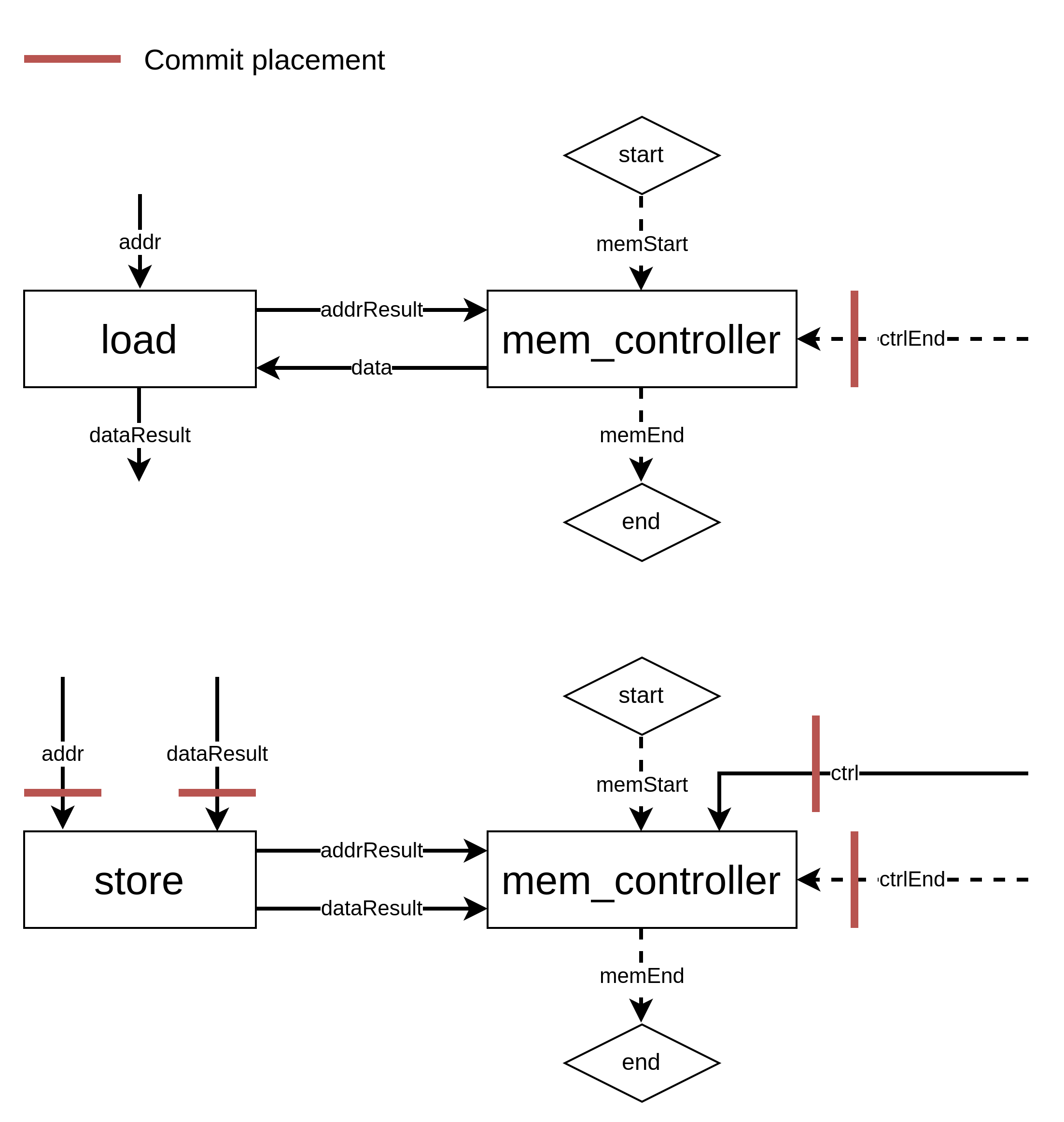
When a memory controller communicates with a LoadOp, five ports of the memory controller are used:
- Two ports for receiving the address from the LoadOp and sending data to the LoadOp
memStart/memEndports, which communicate with external components to signal the start and end of memory region access (see here)- The
ctrlEndport, which receives signals from the control network, indicating that no more requests are incoming.
When the memory controller communicates with a StoreOp, six ports are involved:
- Two ports for receiving the address and data from the StoreOp
memStart/memEnd(as with LoadOp)ctrlEndport (as with LoadOp)ctrlport, which tracks the number of store operations
Commit units are placed on the ctrlEnd and ctrl ports because these ports cause side effects.
Commit units are not placed for the two ports communicating with the LoadOp or StoreOp, nor for the two external ports. For the LoadOp, the communication should happen even if the signal is speculative. For the StoreOp, commit units are already placed in front of the StoreOp, making them redundant here.
How to Place Commit Units for MemoryControllerOp
Our algorithm is designed so that when it visits a MemoryControllerOp, it should place a commit unit. Specifically, at a LoadOp, we skip traversing the results connected to the memory controller.
How does this ensure correct placement?
- Ports connected to a
LoadOpare not traversed due to the skip mentioned above. - Ports connected to a
StoreOpare also not traversed because the traversal stops at theStoreOp. - External ports are never traversed.
- The
ctrlandctrlEndports are traversed if they originate from the speculative region and require a commit unit.
Future Work
This document does not account for cases where Load and Store accesses are mixed in a single memory controller, or where a Load-Store Queue (LSQ) is used. These scenarios are left for future work.
Speculation Integration Tests
The speculation integration tests originate from Haoran’s master’s thesis.
Unlike other integration tests, these require manual modifications to the programs and IR to ensure speculation is effective.
This document explains how to run the speculation integration tests and details the necessary manual modifications.
Running the Tests
There are eight speculation integration tests in the integration-test folder:
single_looploop_pathsubdiagsubdiag_fastfixedsparsenested_loopif_convert(data speculation)
The newton benchmark from Haoran’s thesis is excluded because it contains branches within the loop, where the current speculation approach is ineffective.
Since these tests require manual modifications and a custom compilation flow, we have provided a ready-to-run script. You can execute the speculation integration tests (covering compilation, HDL generation, and simulation) with a single command:
Requirement: Python 3.12 or later is needed to run the script.
$ python3 tools/integration/run_spec_integration.py single_loop
You can run a test without speculation using the custom compilation flow:
$ python3 tools/integration/run_spec_integration.py single_loop --disable-spec
To visualize and confirm the initiation interval, you can simply use the Dynamatic interactive shell:
$ ./bin/dynamatic
> set-src integration-tests/single_loop/single_loop.c
> visualize
Custom Compilation Flow
The full details of the custom compilation flow can be found in the Python script:
tools/integration/run_spec_integration.py.
Below is a summary of its characteristics:
- Compilation starts from the
cfdialect since modifications to the CFG are required under the current frontend (this will be resolved by #311). - The speculation pass (
HandshakeSpeculation) runs after the buffer placement pass. - A custom buffer placement pass follows the speculation pass, just before the
HandshakeToHWpass, ensuring that required buffers for speculation are placed. - We use a Python-based, generation-oriented beta backend, which supports the signal manager.
Each integration test folder contains an input cf file named cf.mlir (e.g., subdiag/cf.mlir).
Even though the compilation flow starts from the cf dialect, the original C program is still required for simulation to generate the reference result.
Maintaining consistency between the C program and the cf IR file is essential—don’t forget!
Manual CFG Modification
Manual modifications to the CFG generated by the frontend are required because:
- Speculation only supports single-basic-block loops.
- The current frontend produces redundant/unexpected CFGs (Issue #311).
Ideally, #311 will eliminate all of the need for these modifications, but some of them are a bit extreme to reduce the number of basic blocks:
-
Convert
whileloops todo-whileloops if the loop is guaranteed to execute at least once. This reduces the basic block handling the initial condition.Before:
while (cond) { // Executed at least once }After:
do { // Executed at least once } while (cond); -
Merge the tail break statement, even in
forloops.Before:
for (int i = 0; i < N; i++) { // Body if (cond) break; }After:
int i = 0; bool break_flag = false; do { // Body i++; break_flag = cond; } while (i < N && !break_flag);
These transformations may not be generally supported, but they help meet the requirements for speculation.
spec.json
Speculation requires some manual configuration, which is defined in the spec.json file located in each integration test folder.
A typical spec.json file looks like this:
{
"speculator": {
"operation-name": "fork4",
"operand-idx": 0,
"fifo-depth": 16
},
"save-commits-fifo-depth": 16
}
Speculator Placement
In this example, the speculator is placed on operand #0 of the fork4 operation. Visually, it is like this:
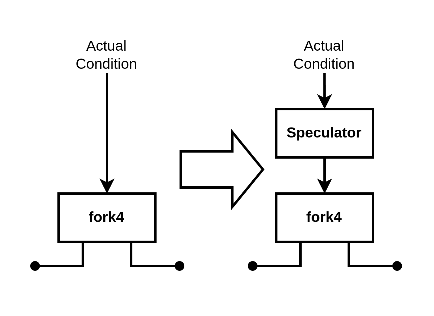
Speculator/Save-Commit FIFO Depth
You also need to specify the FIFO depth for speculator and save-commit units. The FIFO must be deep enough to store all in-flight speculations, from the moment they are made until they are resolved. If the FIFO fills up, the circuit deadlocks.
Note: The save-commits-fifo-depth value is currently shared across all save-commit units.
Buffer Placement
Speculation requires additional buffers to improve initiation interval (II) and prevent deadlocks. Some of these buffers are not placed by the conventional buffering pass since they depend on conditions from the previous iteration.
To handle this, buffers must be manually specified using the existing HandshakePlaceBuffersCustomPass.
This pass takes the following arguments:
pred: Previous operation nameoutid: Result IDslots: Buffer sizetype:"oehb"or"tehb"
Note: Unfortunately, the way buffer positions are specified is opposite to the speculation pass (buffers are placed on results, while speculators are placed on operands).
The buffer configuration is defined in buffer.json under each integration test folder, for example:
[
{
"pred": "fork12",
"outid": 1,
"slots": 16,
"type": "tehb"
},
{
"pred": "speculator0",
"outid": 0,
"slots": 16,
"type": "tehb"
},
...
]
Multiple buffers can be placed, and the custom buffer placement pass is invoked multiple times.
For the first item in the example above, the buffer placement looks like this:
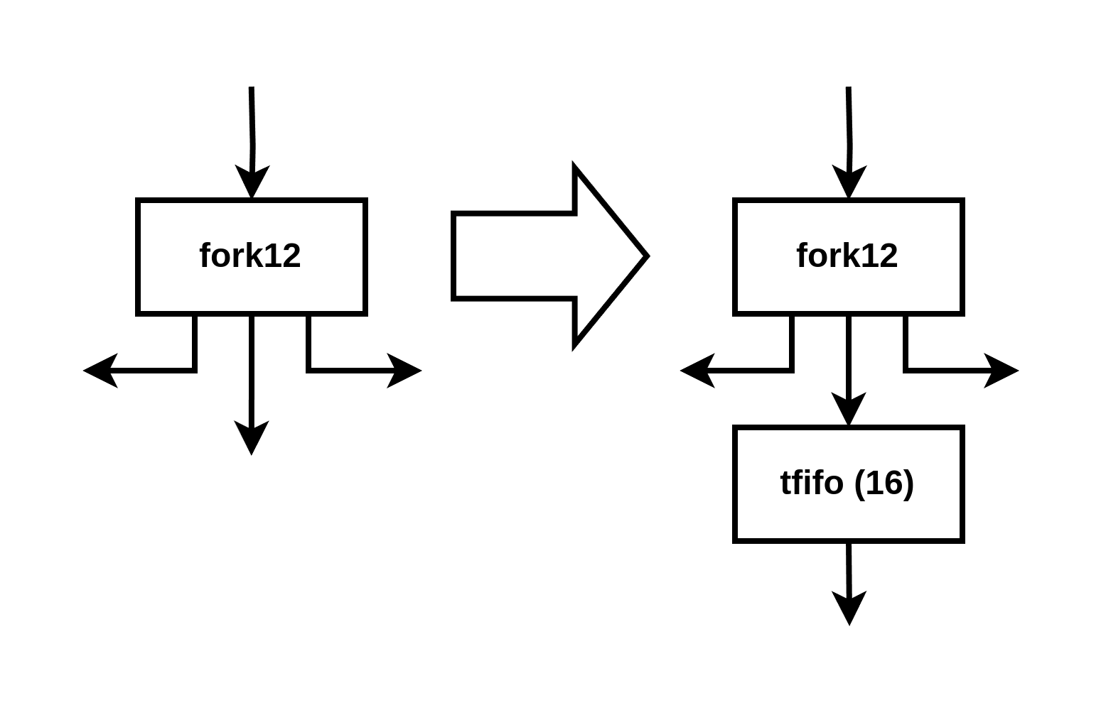
Note: Opinion on Placement Specification
In my opinion, buffer positions should be specified by operand rather than result. Operands are always unique, even without materialization, whereas results are not.
Integration Test Folder
The integration test folders are located at integration-test/(test-name)/. Each folder also contains:
(test-name)_original.c: The original program from the thesis.cfg_modification.png: A diagram illustrating the CFG modifications applied to the program.results.md: The benchmark results.
Save Commit Behavior
The table below illustrates the behavior of the save-commit unit, which is not included in my final report:
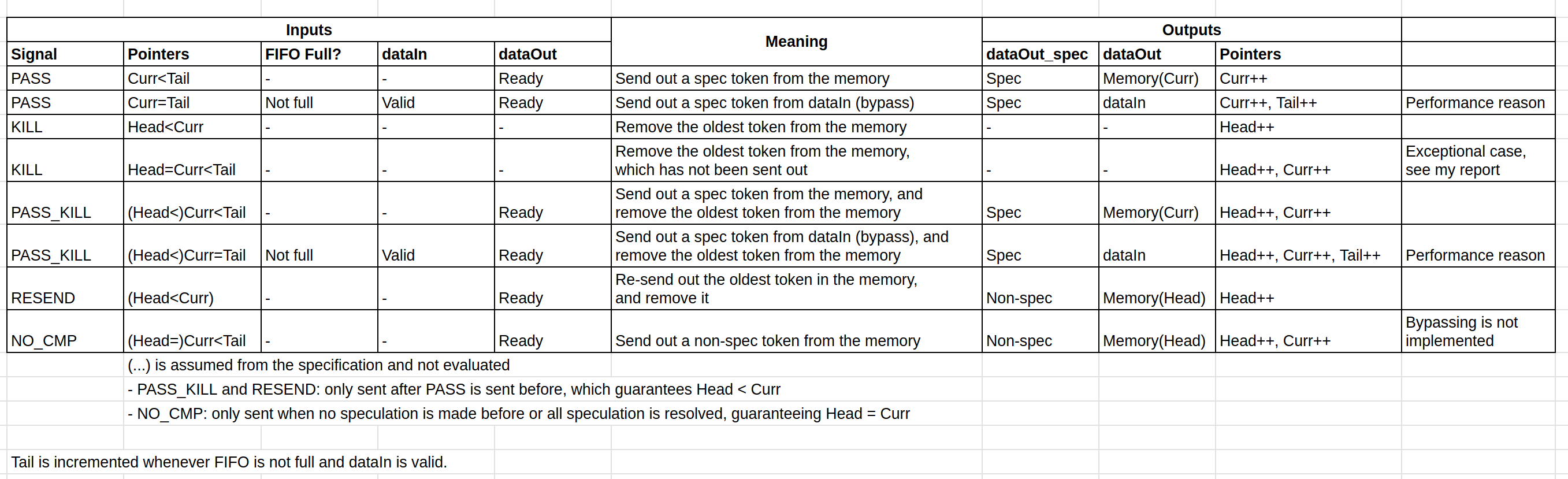
Also see Section 6.3 of my report for the explanation of the save-commit unit’s design.
BLIF Exporter
The BLIF Exporter is an binary that serializes a Synth dialect circuit contained inside hw.module operations into a BLIF file. It serves as the inverse of the BLIF Importer, allowing Dynamatic’s IR to be exported back to a standard BLIF representation for use with external synthesis tools.
Code Structure
The binary export-blif can be called as follows:
./bin/export-blif <input-mlir-file> <output-blif-file>
where input-mlir-file is the file that contains the Synth circuit to be exported and output-blif-file is the file containing the exported BLIF.
The core functionality is the following:
- It iterates over all
hw.HWModuleOpoperations in the module and callsexportBlifCircuiton each of them to generate a BLIF module.
The core function exportBlifCircuit executes the following steps:
- It writes the
.model,.inputs, and.outputslines, and collects all port names into theinputPortsandoutputPortsvectors using thegenerateBlifHeaderfunction. - It iterates over the ops inside the module body and emit the corresponding BLIF statements using the
generateBlifCircuitFromSynthfunction. - Writes the
.endterminator to close the BLIF model.
Support Functions
In this subsection of the doc, we highlight the key support functions.
Generate BLIF Header
The core function that writes the header section of the BLIF file for a given hw.HWModuleOp is generateBlifHeader. It:
- Writes the
.modelline using thehw.modulename. - Iterates over the module’s port list and writes all input ports on the
.inputsline. It populates the vectorinputPortswhich contains the same list. - Iterates over the module’s port list and writes all output ports on the
.outputsline. It populates the vectoroutputPortswhich contains the same list.
Generate BLIF Functionality
The core function that translates the Synth operations inside an hw.HWModuleOp into BLIF statements is generateBlifCircuitFromSynth. It iterates over all ops in the module body and handles three operation types:
-
synth.latch: the function emits a.latchstatement with the format.latch <input> <output> [type control] [init]. The input and output operand names are resolved viagetValueName. Optional fields are emitted only when present: if a control signal exists, the latch type (defaulting to"re"if unset) and control signal name are written; if an init value is set, it is appended. -
synth.aig.and_inv: the function emits a.namesstatement listing both input operand names and the output result name, followed by a truth-table row. Each input position in the row is"0"if that input is inverted and"1"otherwise. -
hw.constant: the function emits a single-node.namesstatement (.names <output>) followed by either1or0on the next line, corresponding to the constant’s value. Only 1-bit constants are supported. -
hw.output: after all ops are processed, the function checks whether any output port is directly connected to an input port (i.e., a pass-through with no Synth op in between). For each such case, a two-node.nameswire statement is emitted (1 1), connecting the input port name to the output port name. At the end, the function asserts that every output port has been accounted for.
Any other operation type is reported as unsupported via an error message.
Value Naming in BLIF
Value names in the BLIF output are resolved by the internal getValueName lambda, which applies the following priority:
- If the value is a block argument (input port), return its name from
inputPortsusing the argument index. - If the value is used as an operand of
hw.output(output port), return its name fromoutputPortsusing the operand index offset by the number of input ports. - Otherwise, print the value using MLIR’s
AsmState(e.g.,%4), strip the leading%, and prependnto produce a valid BLIF node name (e.g.,n4).
This function ensure uniqueness and consistency of names inside a BLIF module.
BLIFFileManager
Overview
BLIFFileManager is a utility class that resolves .blif file paths describing the functionality of Handshake IR operations. Given a base directory and an operation, it constructs the expected file path and validates that the file exists.
File Path Convention
BLIF files are organized by module type and parameters using this structure:
<blifDirPath>/<moduleType><extraSuffix>/<param1>/<param2>/.../<moduleType><extraSuffix>.blif
Example: A fork operation with size 2 and data width 32 would resolve to:
<blifDirPath>/fork_type/2/32/fork_type.blif
Key Functions
combineBlifFilePath
std::string combineBlifFilePath(std::string moduleType,
std::vector<std::string> paramValues,
std::string extraSuffix = "");
Builds the full file path from the module type, a list of parameter values, and an optional suffix.
getBlifFilePathForHandshakeOp
std::string getBlifFilePathForHandshakeOp(Operation *op);
Dispatches on the operation type to extract the relevant parameters and construct the BLIF file path. Returns an empty string for unsupported operations.
If the resolved path does not exist on disk, an error is emitted and an assertion fails.
Supported Operations & Parameters
| Operation(s) | Parameters Used |
|---|---|
AddI, AndI, CmpI, OrI, ShLI, ShRSI, ShRUI, SubI, XOrI, MulI, DivSI, DivUI, Select, SIToFP, FPToSI, ExtF, TruncF | Data width of first operand |
Constant | Data width of result |
Branch, Sink | Data width (or _dataless suffix if 0) |
Buffer | Buffer type + data width (or _dataless if 0) |
ConditionalBranch | Data width of data operand (or _dataless if 0) |
ControlMerge | Number of inputs + index type width (dataless only; data variant unsupported) |
ExtSI, ExtUI, TruncI | Input width + output width |
Fork, LazyFork | Number of outputs + data width (or _dataless if 0) |
Mux | Number of inputs + data width + select width |
Merge | Number of inputs + data width |
Load, Store | Data width + address width |
Source | No parameters |
Error Handling
- If the resolved BLIF file path does not exist, an error is printed to
stderridentifying the operation by its unique name and the expected path. - An assertion then halts execution to prompt investigation of the path construction logic.
- Operations not matched by the type switch silently return an empty string (no file lookup is attempted).
Blif Importer
The BLIF Importer is a binary that reads a BLIF file and generates a corresponding Synth dialect circuit inside an hw.module. It serves as a standalone entry point for importing externally synthesized logic directly into Dynamatic’s IR.
This code interprets each BLIF model as an AIG-style circuit composed of 1-bit registers and AND-with-inverter gates, and re-expresses it directly in the Synth dialect while preserving the instance’s interface.
Code Structure
The binary import-blif can be called as follows:
./bin/export-blif <output-mlir-file> <intput-blif-file>
where output-mlir-file is the file that will contain the Synth circuit to be imported and input-blif-file is the file containing imported BLIF.
The code core function is importBlifCircuit(moduleOp, loc, blifFilePath) which imports the blif specified in blifFilePath in the module operation moduleOp.
This function executes the following steps:
- Extract the module name, input and output port names of the module from the BLIF file using the
getBlifModuleHeaderfunction. - Create an hw module operation
hw.HWModuleOpwith input and output ports corresponding to the one of the model described in the BLIF file using thecreateHWModuleShell. - Create all synth operations inside the
hw.HWModuleOpusing the functionpopulateHWModuleShell. Then, attach all the outputs of the synth circuit to the terminator of thehw.HWModuleOp.
Support Functions
In this subsection of the doc, we highlight the key support functions.
Generate Synth Operations
The core function to generate synth operations is populateHWModuleShell. It parses the BLIF body line by line and emits the corresponding Synth operations. It maintains two maps throughout:
nodeValuesMapwhich maps a BLIF node name to its Synth Value. Pre-populated with all input port signals before parsing begins.tmpValuesMapwhich maps a BLIF node name to a temporaryhw.constant 0placeholder, created when a node’s output is referenced before defining the node. Placeholders are replaced and erased once the real value is available.
IMPORTANT: tmpValuesMap may contain a large number of temporary hw constants which should be cleaned up during synth graph construction. For BLIF generated by tools such as ABC, these temporaries arise primarily from latches since since latches appear at the start of the BLIF file and their inputs are not yet defined at generation time. As a result, performance impact scales mainly with latch count.
It handles two types of units defined in the BLIF:
.latchfrom which it parses input node, output node, and oprtional fields (latchType,controlName,initVal). The optional fields follow the BLIF syntax[type control] [init]and are decoded based on the number of tokens. Asynth.latchof typei1is created and registered viaupdateOutputSynthSignalMappingin order to record its output value..namesfrom which it parses the input and output node names and the truth-table function. Depending on the number of node names, the behaviour is different:
- 1 node name: it is a constant and an
hw.constantis generated - 2 node names: it is a wire or an inverter and it is handled by
createSynthWire - 3+ node names: it is a logic gate and it is handled by
createSynthLogicGate
After parsing, all the outputs of the synth circuit are appended in the synthOutputs variable.
Retrieve the Value of the Input of a BLIF Node
The function that retrieves the input of a synth node is getInputMappingSynthSignal. It resolves a BLIF node name to a Synth Value applying the following steps:
- Return the value from
nodeValuesMapif already defined. - Return the existing placeholder from
tmpValuesMapif one exists. - Create a new
hw.constant 0placeholder, store it intmpValuesMap, and return it.
Save the Value of the Output of a BLIF Node
The function that saves the MLIR Value corresponding to the output of a BLIF node is updateOutputSynthSignalMapping. It registers a newly created Synth value as the definitive signal for a given node name. If a temporary placeholder exists in tmpValuesMap for that name, all its uses are replaced with the new value, its defining hw.constant op is erased, and it is removed from tmpValuesMap. The new value is then recorded in nodeValuesMap.
Create a Wire
The function that creates a wire in the Synth circuit is createSynthWire. It handles two-node .names blocks. Compares the input and output bits of the truth-table function string (format: “X Y”):
- If equal, the output node is aliased directly to the input value via
updateOutputSynthSignalMappingand no new op is created. - If different, a
synth.aig.and_invis created with the input inverted andANDedwith a constant 1, effectively modelling a NOT gate.
Create a Logic Gate
The function that creates a logic gate in the Synth circuit is createSynthLogicGate. It handles multi-input .names blocks. Currently asserts that exactly 2 inputs are present, reflecting that the code operates on already-binarized AIG-form BLIF. The truth-table function string (format: “XY Z”) determines the inversion flags for each input. A synth.aig.and_inv is created with the appropriate inversion flags. If the output bit is 0, a second synth.aig.and_inv ANDing with constant 1 and inverting the first input is appended to negate the result.
Handshake to Synth Conversion Pass
The Handshake to Synth pass (--handshake-to-synth) converts a circuit expressed in the Handshake dialect into an equivalent circuit expressed in the HW and Synth dialects. The output is a hierarchical, gate-level netlist.
The pass requires that every Handshake operation has been annotated beforehand with the path of the BLIF file containing its gate-level implementation. This is done by a separate pass (--mark-handshake-blif-impl). Please refer to this doc for more information.
Invocation
The pass is registered as --handshake-to-synth and operates on a builtin.module containing exactly one non-external handshake.func. It can be applied via dynamatic-opt:
dynamatic-opt --mark-handshake-blif-impl="blif-dir=<path>" \
--handshake-to-synth \
input.mlir -o output.mlir
Overview
The pass executes in two sequential steps, each building directly on the output of the previous one.
Step 1: Unbundle converts every Handshake operation into an hw.module definition and an hw.instance call site inside the top-level hw.module. Handshake’s bundled channel types (!handshake.channel<T>, !handshake.control<>) are split into flat i1 data, valid, and ready signals. Ready signals have their direction flipped relative to data and valid. Multi-bit data channels are split into individual i1 ports. Clock and reset ports are appended to every hw.module. Temporary backedge placeholders (UnrealizedConversionCast ops) bridge forward references during conversion and are eliminated by the end of this step.
Step 2: Populate replaces the synth.subckt placeholder body that Step 1 inserted into each hw.module with the real gate-level netlist imported from the corresponding BLIF file.
Pre-check
Before Step 1 begins, runDynamaticPass() walks every operation inside the handshake.func and asserts that it implements BLIFImplInterface and carries a non-empty BLIF file path. Any operation that fails this check signals a pass failure with an error message directing the user to run --mark-handshake-blif-impl first.
Step 1: Unbundle Handshake types
Conversion flow
unbundleHandshakeChannels() runs the following sequence:
- Locates the single non-external
handshake.funcin the module. - Calls
unbundlePorts()andbuildPortInfoFromHandshakeUnitPorts()to compute the top-levelhw.module’s port list, then creates it withhw::HWModuleOp. - Initializes the
BackedgeBuilderand recordsclkandrstfrom the new module’s block arguments (the last two arguments). - Walks the top-level module’s block arguments in order, calling
saveUnbundledValues()to save inunbundledValuesMapthe map between the hw module block argumentValues with the original handshake function ones. - Iterates over every operation in the function body (skipping
handshake.end) and callsconvertHandshakeOp()for each. - Calls
convertHandshakeFunc()to wire the terminator.
convertHandshakeOp() looks up or creates the hw.module definition for the op via createHWModuleHandshakeOp(), then collects input operands by calling getUnbundledValues() for each input port (inserting pendingValuesMap placeholders for values that have not been created yet), appends clk and rst, and creates an hw.instance. Output results are saved to unbundledValuesMap via saveUnbundledValues(), grouping multi-bit data ports by handshake signal before saving.
convertHandshakeFunc() collects the flat output values for the top module’s terminator by calling getUnbundledValues() for each handshake.end operand (data and valid) and each function argument’s ready signal, sets them on the hw.output terminator, verifies that pendingValuesMap is empty, then erases the handshake.end and handshake.func.
Key data structures
PortKind is a std::variant of three tag structs: DataPortInfo (carrying bitIndex and totalBits), ValidPortInfo, and ReadyPortInfo. It is used throughout Step 1 to distinguish which component of a handshake channel a flat port corresponds to.
HandshakeUnitPort represents a single flat port produced by unbundling. It carries the port name, direction, the original handshake Value it corresponds to, and a PortKind.
UnbundledHandshakeChannel holds the resolved flat Values for a single handshake signal, with named fields dataBits, valid, and ready. It provides setValues(PortKind, SmallVector<Value>) and getValues(PortKind) methods that dispatch on the variant to access the correct field, and an empty() predicate used to detect fully resolved entries.
Type unbundling rules
| Handshake type | Flat components |
|---|---|
!handshake.channel<T> | T (data), i1 (valid), i1 (ready) |
!handshake.control<> | i1 (valid), i1 (ready) |
memref<NxT> | T (data), i1 (valid), i1 (ready) |
| any other type | the type itself (data pass-through) |
Port naming
Port names are derived from NamedIOInterface. For handshake.func the names come directly from the function’s argument and result name attributes. For all other ops, names are obtained from NamedIOInterface::getOperandName / getResultName, then legalized by legalizeBlifPortNames(), which converts the root_N index pattern to root[N] array notation (back-patching root to root[0] when index 1 is first encountered). Signal-kind suffixes are then appended: _valid and _ready are inserted before the first [ for array names, or appended at the end otherwise. Data port names for multi-bit channels use the same formatting rule with a numeric index.
Signal tracking and placeholder resolution
HandshakeUnbundler maintains two maps keyed by handshake Value:
unbundledValuesMap holds the definitive flat Values for each handshake signal, stored as UnbundledHandshakeChannel entries.
pendingValuesMap holds temporary backedge placeholders (UnrealizedConversionCast ops created via BackedgeBuilder) for signals whose producing op has not yet been converted. When saveUnbundledValues() is later called with the real values, it calls replaceAllUsesWith() on each placeholder to redirect uses, then clears the entry. The BackedgeBuilder (owned as std::unique_ptr<BackedgeBuilder>) erases the now-unused placeholder ops in its destructor.
Step 2: Populate hw modules with BLIF netlists
Code structure
Step 2 is implemented by populateHWModule() and the public entry point populateAllHWModules().
populateHWModule() resolves the hw.module definition referenced by a given hw.instance, looks up its BLIF path in opToBlifPathMap, imports the netlist with importBlifCircuit(), then swaps the original module out of the symbol table and inserts the imported one under the same name. A DenseSet<StringRef> of already-populated module names prevents the same module from being imported more than once when multiple instances reference it.
populateAllHWModules() locates the top-level hw.module by name, collects all hw.instance ops it contains via a walk, and calls populateHWModule() for each.
BLIF path lookup
The BLIF path for each module is stored in the global opToBlifPathMap (DenseMap<Operation*, string>), which is written during Step 1 in createHWModuleHandshakeOp(). An empty path means the module’s body should not be replaced.
Global shared state
opToBlifPathMap (DenseMap<Operation*, string>) maps each hw.module operation to the path of the BLIF file that should replace its placeholder body. It is written in Step 1 and consumed in Step 2.
CLK_PORT and RST_PORT are string constants used consistently by Step 1 when building port info and when identifying clock and reset ports during instance operand collection.
HandshakeMarkBLIFImpl Pass
Overview
HandshakeMarkBLIFImpl is a pass that annotates every Handshake operation in a module with the path to its corresponding .blif implementation file. These annotations are later consumed by the Handshake to Synth conversion pass.
The pass uses BLIFFileManager to resolve file paths and attaches them to operations via the BLIFImplInterface.
Pass Behaviour
- Validates that the
blifDirPathoption is non-empty; fails the pass otherwise. - Instantiates a
BLIFFileManagerwith the provided directory path. - Walks all operations in the module, skipping
handshake::FuncOp. - For each operation, resolves the BLIF file path using
BLIFFileManager::getBlifFilePathForHandshakeOp. - Annotates the operation by calling
BLIFImplInterface::setBLIFImplwith the resolved path.
Options
| Option | Type | Description |
|---|---|---|
blifDirPath | string | Base directory containing all .blif files. Must be non-empty. |
BLIFImplInterface
An MLIR OpInterface that allows any Handshake operation to carry a reference to its BLIF implementation.
The interface stores the BLIF path as a StringAttr under the attribute name "blif_impl".
Methods
setBLIFImpl(StringRef value)
Sets the "blif_impl" attribute on the operation to the given string value.
getBLIFImpl() → StringAttr
Returns the "blif_impl" attribute. If the attribute is not set, returns an empty StringAttr.
Example Attribute
After the pass runs, an annotated operation will carry an attribute such as:
blif_impl = "/path/to/blif/fork_type/2/32/fork_type.blif"
Synth dialect
The Synth dialect is a low-level synthesis-oriented dialect that provides a common in-MLIR interface for logic synthesis operations and data structures. It is intended as an intermediate representation between higher-level hardware IR (e.g., Handshake or HW) and concrete synthesis backends, capturing both logic networks (such as AIGs) and meta-operations that steer synthesis decisions.
In Dynamatic, operations of the synth dialect are always described inside an hw.module operation of the hw dialect.
Design and role in the flow
The Synth dialect has a core responsibility:
- Support logic network representations such as AIG (And-Inverter Graph) and sequential elements as latches.
In other words, the Synth dialect is not tied to a particular hardware backend or HDL; instead, it serves as an abstraction layer where logic-level manipulations can be expressed, analyzed, and transformed before being committed to a specific RTL or gate-level format.
Operations
This dialect describes two core operations:
AndInverterOpwhich describes the nodes of an AIG.LatchOpwhich describes the presence of a latch.
And-Inverter Node
It represents a node in an AIG. It computes the bitwise AND of all inputs, each of which may be individually inverted.
%r1 = synth.aig.and_inv %a, %b : i1
%r2 = synth.aig.and_inv not %a, %b : i1
%r3 = synth.aig.and_inv not %a, not %b : i1
Latch Node
It models a storage element, directly corresponding to the BLIF .latch construct. Accepts three optional parameters: a latchType string (“fe”, “re”, “ah”, “al”, “as”), a control clock/enable signal, and an initVal encoding the initial state (0, 1, 2 = don’t care, 3 = unknown).
%q = synth.latch %d : i1
%q = synth.latch %d clock %clk init 0 : i1
Floating Point Units
This document explains the integration of floating-point units in Dynamatic. Dynamatic relies on external frameworks to generate efficient floating-point units. The current version of Dynamatic supports floating-point units from two generators:
How to Specify the Unit Generator?
In order to specify which units to use, the user can use the following command when executing dynamatic:
set-fp-units-generator generator_name
For instance, here is a complete script used in Dynamatic’s frontend that uses the floating-point units generated by Flopoco:
set-dynamatic-path .
set-fp-units-generator flopoco
set-src integration-test/fir/fir.c
compile
write-hdl
simulate
synthesize
exit
Dynamatic uses flopoco by default.
Important: Using Vivado’s Floating Point Units
Vivado’s floating point units are proprietary. Therefore, we need to compile the modelsim simulation library using Vivado, and point Dynamatic to the location of the simulation library and the installation path of Vivado.
Compiling Simulation Library for ModelSim
To use the floating point units provided by Vivado, we need to compile them using Vivado. In Vivado, select Tools -> Compile simulation libraries -> ModelSim simulator, and set the path to where your ModelSim is (see the screenshot below).
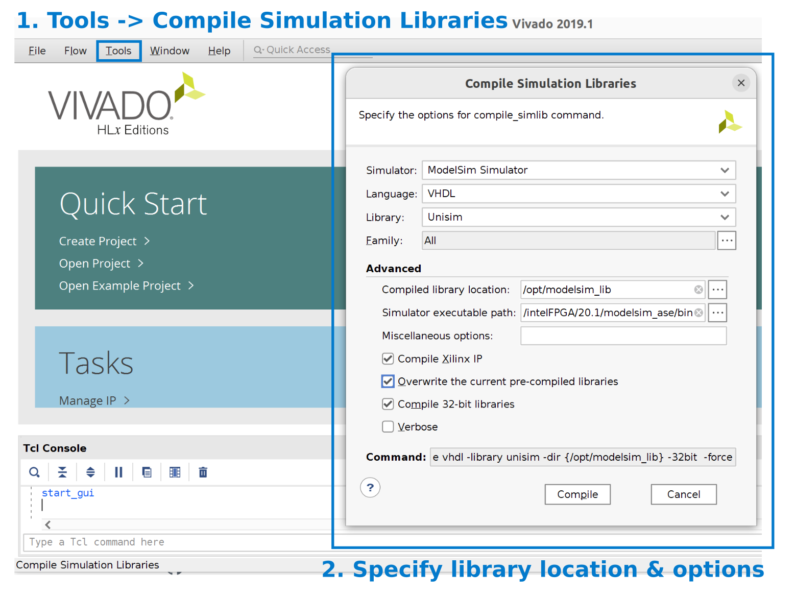
Please refer to this link for more information on how to compile the simulation library for ModelSim.
Make sure that you have compatible versions of Vivado and ModelSim. The following link contains a list of compatible versions: https://www.xilinx.com/support/answers/68324.html
Once the user has downloaded the Vivado IPs, the user has to update the path of these libraries for modelsim simulation by updating the path /opt/modelsim_lib/ in this modelsim.ini.
Important: Extra setup for Vivado
Additionally, the user has to provide the path to the Vivado installation folder using set-vivado-path. Here is a complete script for Dynamatic’s frontend:
set-dynamatic-path .
# Installation path of Vivado
set-vivado-path /path/to/vivado/Vivado/2019.1
set-fp-units-generator flopoco
set-src integration-test/fir/fir.c
compile
write-hdl
simulate
synthesize
exit
The default value for the vivado path is /tools/Xilinx/Vivado/2019.1/. This information is essentially to correctly integrate necessary simulation files of Vivado.
RTL and Timing Information
This section describes the organization of RTL modules and the delay/latency information of the floating point units inside Dynamatic.
Dynamatic wraps the floating-point IPs with handshaking logic. Currently, the IP cores are extracted and wrapped in handshake wrappers offline, and we save them in:
# Handshake units with flopoco IP cores:
data/vhdl/arith/flopoco/*.vhd
# Handshake units with Vivado IP cores:
data/vhdl/arith/vivado/*.vhd
The same applies to the Verilog backend where the paths are data/verilog/arith/flopoco/*.vhd and data/verilog/arith/flopoco/*.vhd, respectively.
Internally, Dynamatic uses two sets of files to track how they are generated and the delay/latency properties of them:
- Units with Flopoco IP cores: rtl-config-vhdl-flopoco.json (for RTL generation) and components-flopoco.json (for retreiving the delay/latency values).
- Unist with Vivado IP cores: rtl-config-vhdl-vivado.json (for RTL generation) and components-vivado.json (for retrieving the delay/latency values).
For more information related to timing information, please refer to this markdown.
IMPORTANT: Flopoco does not currently generate Verilog code. When the Flopoco FPU units are specified, the Verilog backend uses VHDL file which have been modified to adapt to Verilog. Hence, there is a mixed-language (VHDL and Verilog) generation.
IMPORTANT: The files used for simulation of the Vivado IPs are specified in VHDL for Modelsim. Hence, when simulating the Verilog modules, the core IP function is specified in VHDL. Hence, there is a mixed-language (VHDL and Verilog) simulation.
Performance comparison : FloPoCo vs Vivado
This section presents some reference side-by-side comparisons of operating frequency and ressource usage for common 32-bit operators, between FloPoCo and Vivado.. All the data presented was obtained by perfoming a place and route in Vivado 2019.1 and using the provided timing and utilsiation reports.
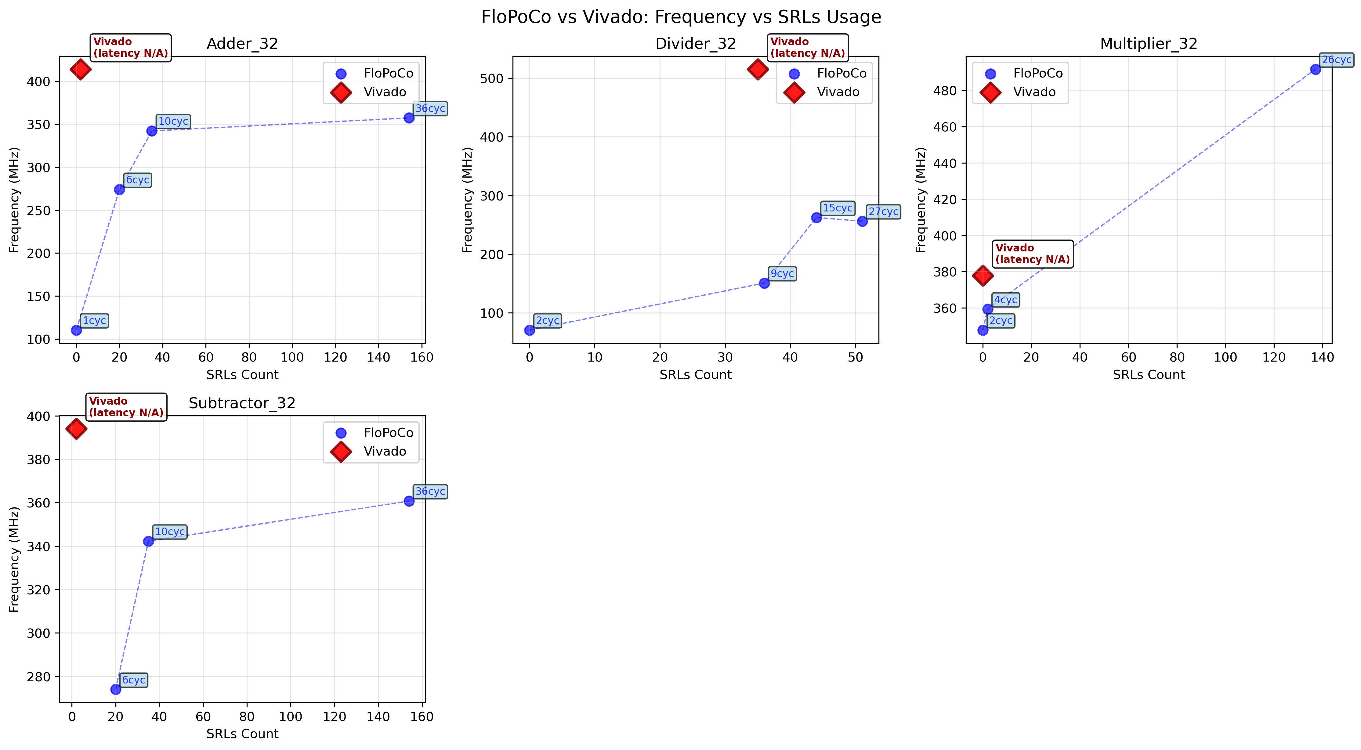
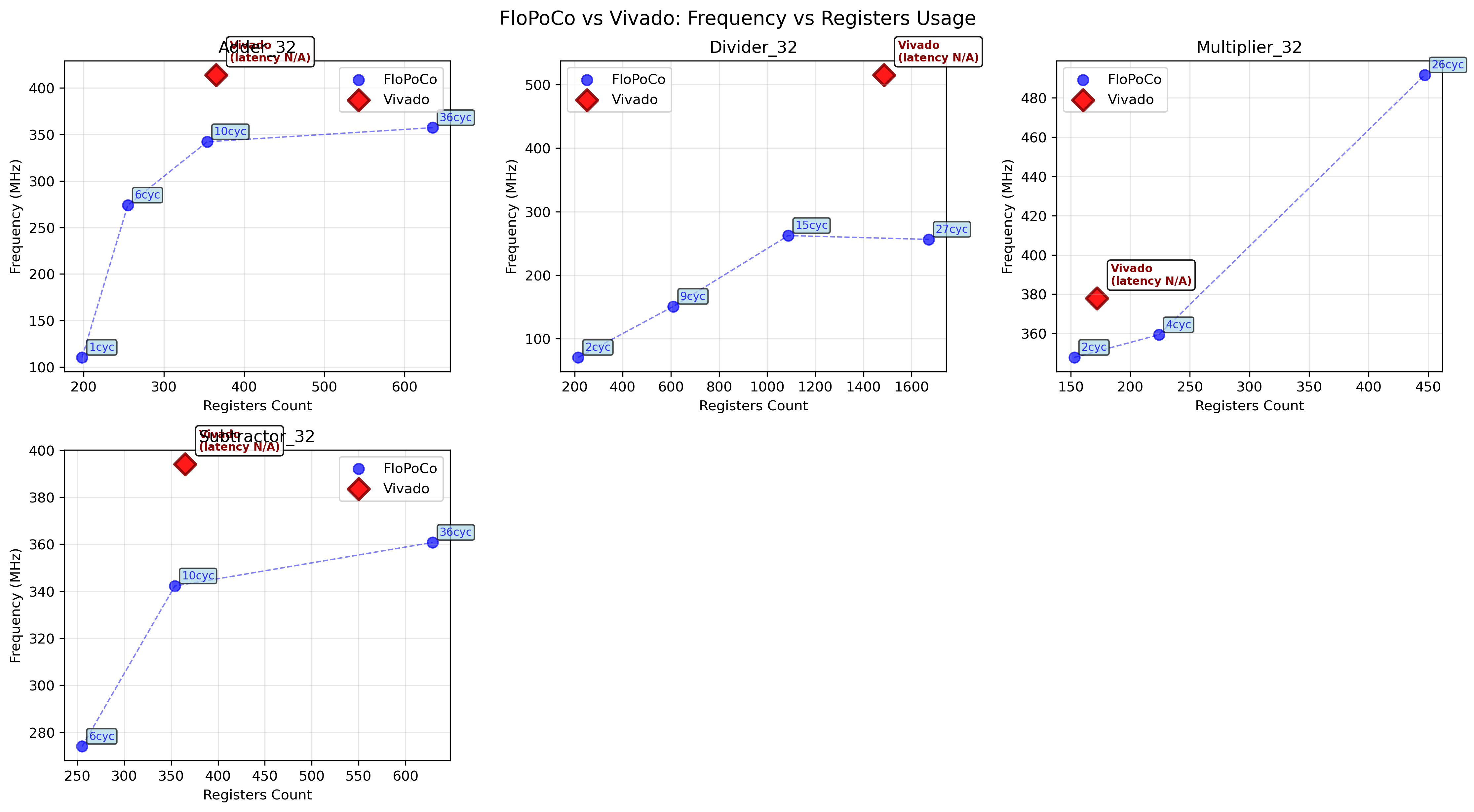
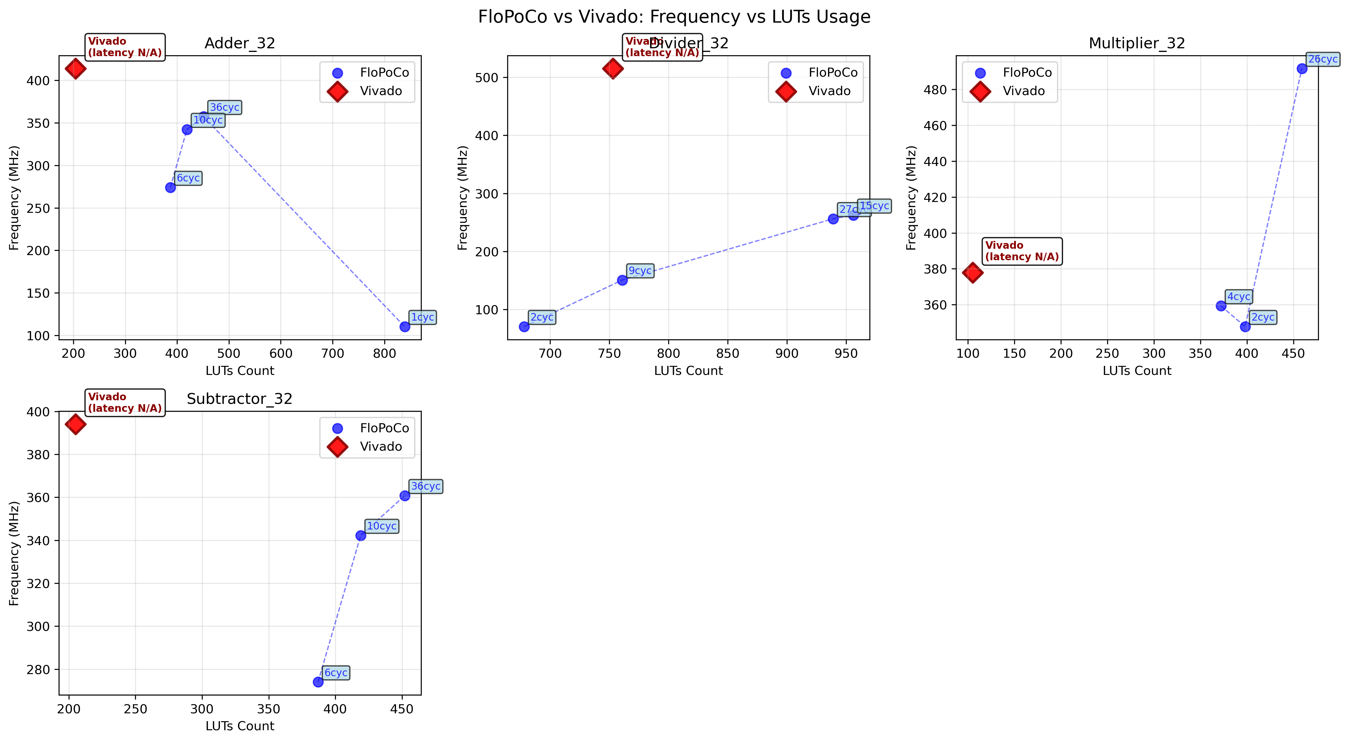
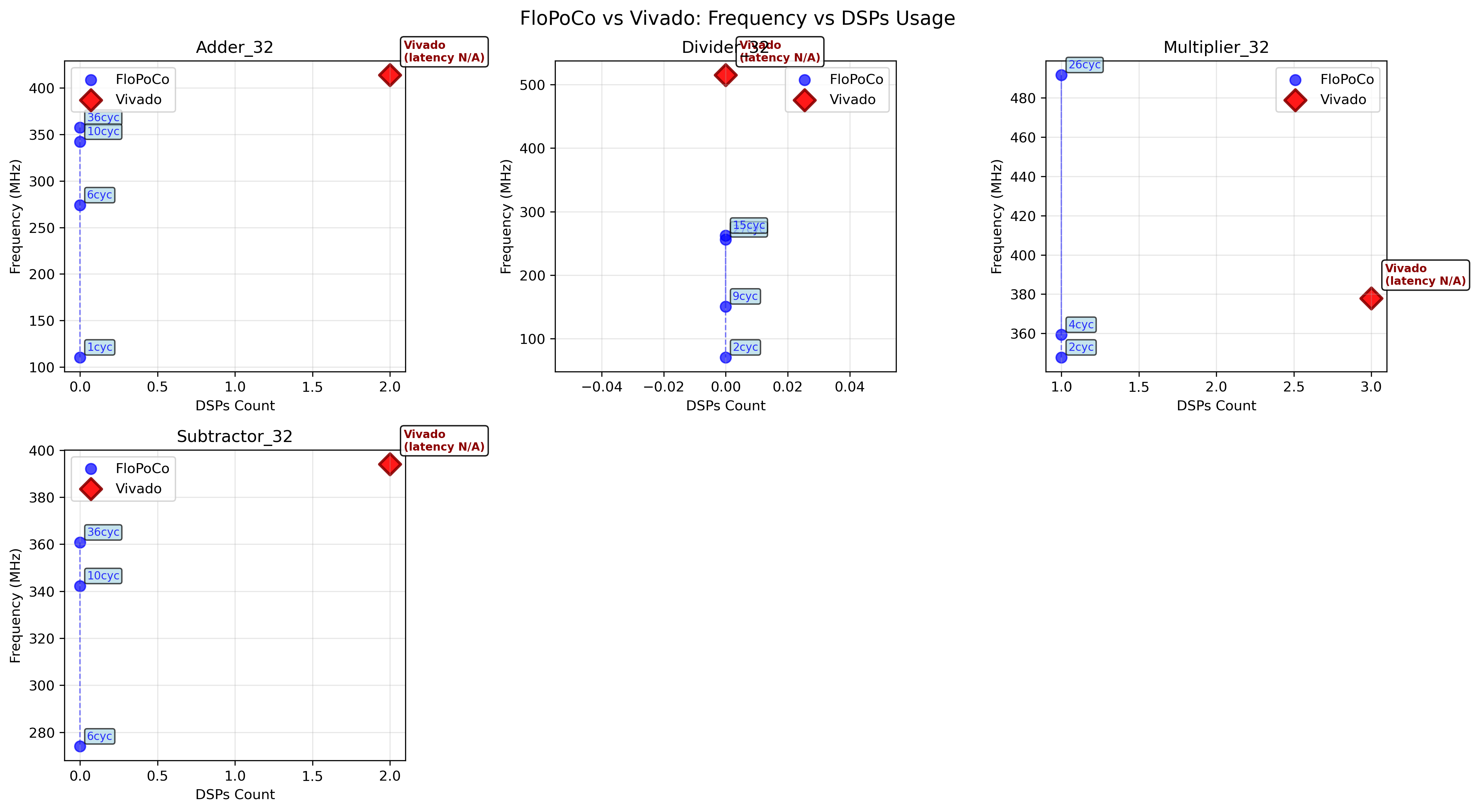
HW Flatten Modules Pass
The HW Flatten Modules pass inlines all hw.instance operations into their
parent hw.module, replacing each instance with the body of the referenced
module. After inlining, the now-redundant module definitions are erased, leaving
a single flat hw.module per top-level circuit.
Overview
The pass operates on a builtin.module containing one or more hw.module
operations, some of which instantiate others via hw.instance. After the pass
runs, no hw.instance ops remain and every module that was instantiated has
been removed.
The pass can be invoked as follows:
./bin/dynamatic-opt --flatten-modules <input-mlir-file>
Code Structure
The core logic lives in FlattenModulesPass::runOnOperation() and proceeds in
three phases:
-
Record instantiated modules. Before any inlining, the pass walks all
hw.instanceops and records the name of every referenced module. This snapshot is used later to decide which modules to erase. -
Inline all instances. The pass repeatedly walks the IR looking for
hw.instanceops. Each time one is found, the body of the referencedhw.moduleis inlined at the call site using MLIR’sinlineRegionutility, and the instance op is erased. The walk restarts after each mutation and continues until no instances remain. -
Erase inlined modules. Any
hw.modulewhose name was recorded in step 1 is erased from the top-level module, as its definition is no longer needed.
Support: HWInliner
The HWInliner struct subclasses MLIR’s InlinerInterface and provides the
inlining policy used in step 2. It implements three methods:
-
isLegalToInline(Region*, ...): always returnstrue, since inlininghw.modulebodies is always legal in this context. -
isLegalToInline(Operation*, ...): always returnstruefor the same reason. -
handleTerminator: called when the inliner encounters thehw.outputterminator of the inlined module. It wires each output value back to the corresponding result of the originalhw.instanceop by replacing all uses.
Limitations
- The pass inlines all instances unconditionally. There is no heuristic to skip large or stateful modules.
- Only
hw.instanceops targetinghw.moduledefinitions are inlined. Instances targetinghw.module.externor other module-like ops are silently skipped.
Dataflow Unit Characterization Script Documentation
This document describes how Dynamatic obtains the timing characteristics of the dataflow units. Please check out this doc if you are unfamiliar with Dynamatic’s timing model.
Dynamatic uses a Python script to obtain the timing characterization.
NOTE: The script and the following documentation are tailored for the specific version of Dynamatic and the current status of the structure of the timing information file. When generating new dataflow units, try to follow the same structure as other dataflow units (in the timing information file and in the VHDL definition). This would make it possible to extend the characterization to new dataflow units.
What is Unit Characterization?
Unit characterization refers to the systematic process of evaluating hardware units (e.g., VHDL modules) for various configurations. The script supports:
- Parameter Sweeping: Automatically varying generic parameters (e.g., bitwidth, depth) and generating the corresponding testbenches and synthesis scripts.
- Dependency Resolution: Ensuring all required VHDL files and dependencies are included for synthesis.
- Parallel Synthesis: Running multiple synthesis jobs concurrently to speed up characterization.
- Automated Reporting: Collecting and organizing timing and resource reports for each configuration.
How to Use the Script
- Prepare VHDL and Dependency Files Ensure all required VHDL files and dependency metadata are available.
- Configure Parameters
Update
parameters_rangesfor the units you wish to characterize. - Run Characterization
Call
run_unit_characterizationfor each unit, specifying the required directories and tool. - Analyze Results Timing and synthesis reports are generated for each parameter combination and stored in the designated report directory.
How to Run Characterization
An example on how to call the script is the following one:
python main.py --json-output out.json --dynamatic-dir /home/dynamatic/ --synth-tool "vivado-2019 vivado"
which would save the output JSON file in out.json which contains timing information, it would specify the dynamatic home directory as /home/dynamatic/ and it would call vivado using the command vivado-2019 vivado. An alternative call is the following one:
python main.py --json-output out.json --dynamatic-dir /home/dynamatic/ --synth-tool "vivado-2019 vivado" --json-input struct.json
where the only key difference is the specification of the input JSON (struct.json) which contains information related to RTL characteristics of each component. If unspecified, the script will look for the following file DYNAMATIC_DIR/data/rtl-config-vhdl-vivado.json.
Overview
The script automates the extraction of VHDL entity information, testbench generation, synthesis script creation, dependency management, and parallel synthesis execution. Its primary goal is to characterize hardware units by sweeping parameter values and collecting synthesis/timing results.
Where Characterization Data is Stored
All generated files and results are organized in a user-specified directory structure:
- HDL Output Directory: Contains all generated/copy VHDL files for each unit and configuration.
- TCL Directory: Stores synthesis scripts for each configuration.
- Report Directory: Contains timing and resource reports produced by the synthesis tool.
- Log Directory: Stores log files for each synthesis run.
Each configuration (i.e., a unique set of parameter values) is associated with its own set of files, named to reflect the parameter values used.
Scripts Structure
The scripts are organized according to the following structure:
.
├── hdl_manager.py # Moves HDL files from the folder containing all the HDL files to the working directory
├── report_parser.py # Extracts delay information from synthesis reports
├── main.py # Main script: orchestrates filtering, generation, synthesis, parsing
├── run_synthesis.py # Runs synthesis (e.g., with Vivado), supports parallel execution
├── unit_characterization.py # Coordinates unit-level processing: port handling, VHDL generation, exploration across all parameters
└── utils.py # Shared helpers: common class definitions and constants
Core Data Structures and Functions
The scripts uses several key functions and data structures to orchestrate characterization:
Parameter Management
-
parameters_ranges: (File
utils.py)A dictionary mapping parameter names to lists of values to sweep. Enables exhaustive exploration of the design space.
Entity Extraction
-
extract_generics_ports(vhdl_code, entity_name): (File
unit_characterization.py)Parses VHDL code to extract the list of generics (parameters) and ports for the specified entity.
- Removes comments for robust parsing.
- Handles multiple entity definitions in a single file.
- Returns:
(entity_name, VhdlInterfaceInfo).
-
VhdlInterfaceInfo: (File
utils.py)A class that contains information related to generics and ports of a VHDL module
Testbench Generation
-
generate_wrapper_top(entity_name, VhdlInterfaceInfo, param_names): (File
unit_characterization.py)Produces a VHDL testbench wrapper for the entity, with generics mapped to parameter placeholders.
- Ensures all generics are parameterized.
- Handles port mapping for instantiation.
Synthesis Script Generation
-
UnitCharacterization: (File
utils.py)A class that contains information related to parameters used for a characerization and the corresponding timing reports.
-
write_tcl(top_file, top_entity_name, hdl_files, tcl_file, sdc_file, rpt_timing, VhdlInterfaceInfo): (File
utils.py)Generates a TCL script for the synthesis tool (e.g., Vivado), including:
- Reading HDL and constraint files.
- Synthesizing and implementing the design.
- Generating timing reports for relevant port pairs.
-
write_sdc_constraints(sdc_file, period_ns): (File
run_synthesis.py)Creates an SDC constraints file specifying the clock period.
Dependency Handling
-
get_hdl_files(unit_name, generic, generator, dependencies, hdl_out_dir, dynamatic_dir, dependency_list): (File
hdl_manager.py)Ensures all required VHDL files (including dependencies) are present in the output directory for synthesis.
Synthesis Execution
-
run_synthesis(tcl_files, synth_tool, log_file): (File
run_synthesis.py)Runs synthesis jobs in parallel using the specified number of CPU cores.
- Each job is executed with its own TCL script and log file.
-
_synth_worker(args): (File
run_synthesis.py)Worker function for executing a single synthesis job.
Report Parsing
-
extract_rpt_data(map_unit_to_list_unit_chars, json_output): (File
report_parser.py)Extract data from the different reports and it saves it into the
json_outputfile. The datamap_unit_to_list_unit_charscontains a mapping between unit and a list of UnitCharacterization objects. Please look at the end of this doc to find an example of the structure of the expected report.
High-Level Flow
-
run_unit_characterization(unit_name, list_params, hdl_out_dir, synth_tool, top_def_file, tcl_dir, rpt_dir, log_dir): (File
unit_characterization.py)Orchestrates the full characterization process for a single unit:
- Gathers all HDL files and dependencies.
- Extracts entity information and generates testbench templates.
- Sweeps all parameter combinations, generating top files and TCL scripts for each.
- Runs synthesis and collects reports.
- Returns a mapping from report filenames to parameter values.
Using a New Synthesis Tool
For now the code has some specific information related to Vivado tool. However, adding support for a new backend should not take too long. Here it is a list of places to change to use a different backend:
_synth_worker-> This function runs the synthesis tool. It assumes the tool can be called as follows:SYNTHESIS_TOOL -mode batch -source TCL_SCRIPT.write_tcl-> This function writes the tcl script with tcl commands specific of Vivado.write_sdc_constraints-> This function writes the sdc file and it is tailored for Vivado. It might also require some changes.PATTERN_DELAY_INFO-> This is a constant string used to identify the line where the report specifies the delay value. This is tailored for Vivado.extract_delay-> This function extracts the total delay of a path from the reports. This is tailored for Vivado.
These files might require some changes if the synthesis tool has different features from Vivado.
Example: Parameter Sweep and Synthesis
Suppose you want to characterize a FIFO unit with varying depths and widths. You would set up parameters_ranges as follows:
parameters_ranges = {
"DEPTH": [8, 16, 32],
"WIDTH": [8, 16, 32]
}
The script will automatically:
- Generate all combinations (e.g., DEPTH=8, WIDTH=8; DEPTH=8, WIDTH=16; …).
- For each combination, generate a top-level testbench, TCL script, and SDC constraints.
- Run synthesis for each configuration in parallel.
- Collect and store timing/resource reports for later analysis.
Example: Expected Report Structure
The synthesis report is expected to contain this line Data Path Delay: DELAY_VALUEns which is used to extract its delay.
Please refer to Using a New Synthesis Tool section if the lines containing ports and delays information are different in your report.
Notes
- The script is designed for batch automation in hardware design flows, specifically targeting VHDL and Xilinx Vivado.
- It assumes a certain structure for VHDL entities and their dependencies.
- Parallelization is controlled by the
NUM_CORESvariable. - The script can be extended to support additional synthesis tools or more complex dependency structures.
XLS Integration
Overview
XLS is an open-source, data-flow oriented HLS tool developed by Google, with quite a potential for synergy with Dynamatic: In short, Dynamatic is very good at designing networks of data flow units, while XLS is very good at synthesizing and implementing arbitrary data flow units.
Very recently XLS gained an MLIR dialect and interface, greatly simplifying potential inter-operability between the two.
This MLIR dialect is available in Dynamatic if enabled at compilation
(--experimental-enable-xls flag in ./build.sh).
This documents serves as an overview of this integration, because due some unfortunate points of friction, it is not quite as straight forward as one might hope.
Challenges
Specifically, integration is hindered by two issues:
-
XLS uses the
bazelbuild system, and does not rely on the standard MLIR CMake infrastructure. As such, it has a very different project and file structure, that does not cleanly integrate in Dynamatic. -
XLS is religiously updated to the newest version of LLVM, with new upstream versions often being pinned multiple times a day, while Dynamatic is stuck on the LLVM version used by Polygeist, which is more than two years out of date.
Goals
In this light, the integration was designed with the following in mind:
-
Be opt-in: Since XLS is quite a large dependency and the integration is built on somewhat shaky ground, it is completely disabled by default. This hopefully prevents friction during “mainline” Dynamatic development.
-
Rely on upstream XLS as much as possible: While it is currently impossible to use a “vanilla” checkout of XLS, the amount of patching of XLS code is kept to a minimum and done in a fashion that (hopefully) enables relatively simple updating to a new version of XLS.
-
Be isolated: Minimize the amount of toggles/conditional code paths required in “mainline” XLS tools like
dynamatic-optto handle the presence/absence of XLS.
The Gory Details
Pulling-in XLS
Since XLS is quite large, it is not included as a git submodule as this would see it downloaded by default, even if not required.
Instead, the build.sh script fetches the correct version of XLS to xls/ if
XLS integration is enabled during configuration.
While building, the build.sh script verifies that the xls/ checkout is
at the correct commit/version. If this is not the case, it will print a warning
message but it will not automatically update to the correct version to avoid
deleting work.
The upstream XLS git URL and commit hash are set in build.sh. Note that we
use a fork1 of XLS with minimal compatibility changes. See below.
Conditional Inclusion
If XLS is enabled, build.sh sets the CMake variable DYNAMATIC_ENABLE_XLS
which is in turn is used to enable XLS-specific libraries and targets. This also
causes the DYNAMATIC_ENABLE_XLS macro to be defined for all C++ and Tablegen
targets to allow for conditional compilation.
General Structure
XLS-specific passes were simply added to normal XLS pass sets (like Conversion/Passes.td,
or experimental’s Transforms/Passes.td) and gates using DYNAMATIC_ENABLE_XLS,
this will still require all dynamatic tools and libraries that uses these passes
to link against the XLS dialect if DYNAMATIC_ENABLE_XLS is set. While the dialect
is not particularly large, this would CMakeLists.txt all over Dynamatic.
Instead, all XLS-specific passes, dialects, and code is placed in its own
folder hierarchy (located at experimental/xls), featuring its own include,
folder, Pass sets, and namespace (dynamatic::experimental::xls).
With this setup, only tools that explicitly require XLS features and import
headers from this hierarchy need to link against the XLS dialect and passes
when DYNAMATIC_ENABLE_XLS is set.
This subsystem also features a dedicated test suite that can be run
using ninja check-dynamatic-xls.
Overcoming LLVM Version Differences
Just like any other dialect, the XLS MLIR dialect consists of Tablegen definition (the “ODS”) and C++ source files. Both are naturally written against the up-to-date version of LLVM used by XLS.
To enable translation, we require at least one binary that includes both the Handshake and XLS dialect specification. Because it lives in the Dynamatic repo, this integration takes the route of back-porting the MLIR dialect to the version of LLVM used in Dynamatic.
This means we must compile the Tablegen ODS with our 2023 version of
mlir-tblgen, which does not work out of the box due to small changes in the
ODS structure of the years. For example, the XLS ODS triggers an mlir-tblgen
bug that is fixed upstream but not available in our version 2.
Similarly, we need to compile and link the dialect source files against our version of LLVM, which features slightly different APIs.
To overcome this, we use a fork1 of XLS with a small set of patches that
work around these differences conditionally if the DYNAMATIC_ENABLE_XLS macro
is present.
For example, in Dynamatic’s LLVM version, LogicalResult lives in mlir/, while
in upstream LLVM it has been moved to llvm/:
#ifdef DYNAMATIC_ENABLE_XLS
// Header name changed in LLVM
#include "mlir/include/mlir/Support/LogicalResult.h"
#else
#include "llvm/include/llvm/Support/LogicalResult.h"
#endif // DYNAMATIC_ENABLE_XLS
The conditionally inclusion of all these fixes keeps the patched version compatible
with XLS, allowing the correct version of XLS to be built inside
xls/ if desired.
It is suprising how few changes are needed to get this to compile and pass a first smoke test, given that there are 50’000+ commits between the two LLVM versions. Still, this is not a good and permanent solution. There is a very high likelyhood that there are subtle (or even not so subtle) changes in behaviour that do not prevent the dialect from compiling change its semantics.
Notes
Updating XLS
To pin a new version of XLS, the steps are roughly as follows:
- Pull new XLS commits from upstream to the
mainof the XLS fork1. - Check-out the XLS commit which you wish to pin:
git checkout <HASH> - Create a new
dynamatic_interopbranch at this commitgit checkout -b "dynamatic_interop_$(date '+%Y_%m_%d')" - Re-apply the patches from the previous
dynamatic_interopbranch on your new branch:
Note that you potentially have to update the patches to be compatible with the new version of XLS.git cherry-pick <HASH OF PREVIOUS PATCH COMMIT> - Validate that the XLS+Dynamatic integration works with this new version and patch set.
- Push the new
dynamatic_interopbranch to our fork. - Update
XLS_COMMITinbuild.shto the hash of last commit if your new branch.
Note that we intend to keep the previous integration branches and patch sets around (hence the new branch with date). This ensures that the XLS version and patch set combination relied on by older versions of dynamatic remain available.
Lower Handshake to XLS
Overview
The experimental --lower-handshake-to-xls pass is and
exploratory/proof-of-concept alternative backend for Dynamatic, that converts a
handshake function into a network of XLS “procs” connected by XLS channels.
This network can then be elaborated, converted to XLS IR, and synthesized into Verilog.
The rough flow is as follows:
# Convert final handshake to XLS MLIR:
dynamatic-xls-opt --lower-handshake-to-xls handshake_export.mlir > sprocs.mlir
# Elaborate XLS MLIR:
xls_opt --elaborate-procs --instantiate-eprocs --symbol-dce sprocs.mlir > procs.mlir
# Convert XLS MLIR to XLS IR:
xls_translate --mlir-xls-to-xls procs.mlir --main-function="NAME_OF_TOP_PROC_IN_PROCS_MLIR" > proc.ir
# Optimize:
opt_main proc.ir > proc.opt.ir
# Codegen:
codegen_main proc.opt.ir \
--multi_proc \
--delay_model=asap7 \
--pipeline_stages=1 \
--reset="rst" \
--materialize_internal_fifos \
--flop_inputs=true \
--flop_inputs_kind=zerolatency \
--flop_outputs=true \
--flop_outputs_kind=zerolatency \
--use_system_verilog=false > final.v
Note that the XLS MLIR dialect features a higher-level representation of XLS procs than the
normal XLS IR, called “structural procs” or “sprocs”. These make it much simpler to define
and manipulate hierarchical networks of procs. The --lower-handshake-to-xls pass
emits such sprocs, requiring xls_opt’s --elaborate-procs and --instantiate-eprocs
to convert the MLIR into a form that can be translated to XLS IR.
Implementation
The pass is roughly similar structure to the RTL export of Dynamatic. Since there are no parametric procs in XLS IR, a C++-based code emitter generates proc definitions of all required handshake unit parametertrizations. These are then instantiated and connect in a top proc using XLS channels.
Buffers are not converted to XLS procs, but rather modify the properties of the XLS channels they are replaced by.
Limitations
Note that this is not intended as a working Dynamatic backend, but rather as an exploration of XLS inter-op. Only a subset of handshake ops are supported, and the code is not well tested.
XLS also does not provide fine enough per-proc pipelining control to guarantee that all procs behave equivalent to the verilog/VHDL implementations in terms of latency and transparency.
Dynamatic’s LazyForkOp cannot be represented as an XLS proc, since the later
does not allow a proc to check if an output is ready without sending.
XLS supports floating point operations, but currently no floating point handhsake units are converted: In XLS, at the IR level, there is no notion of floating point arithmetic, and all floating point operations are implemented using a large network of integer/basic ops by the DSLX frontend. This makes writing the parametric emitter for these ops not any more difficult, but certainly much more verbose and annoying.
Known Issues
Blows up if an SSA value is used before it is defined, making loops impossible:
module {
handshake.func @foo() -> (!handshake.channel<i3>) attributes {argNames = [], resNames = ["out0"]} {
%1 = constant %0 {handshake.bb = 1 : ui32, value = 3 : i3} : <>, <i3>
%0 = source {handshake.bb = 1 : ui32} : <>
end {handshake.bb = 1 : ui32} %1 : <i3>
}
}
(Did I mention this was a half-backed proof of concept?)